Changes in the Demand for Labor

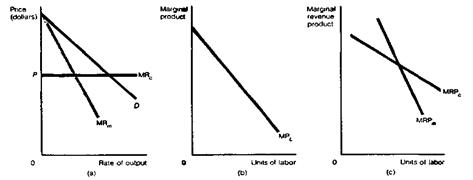
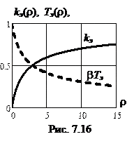
In applying the law of demand to labor, we have seen some adjustments at the firm level and at the industry level in response to wage rate changes. An increase in wage rate changed the price of the product, the employment of other inputs, and the number of firms. However, in establishing the demand curve for labor, many other things were held constant, such as the demand for the product, the prices of other inputs, and the level of technology. If these things were not held constant, then we would not have been able to establish the relation atwage rate to the amount of labor demanded.

1 If the demand for the product that labor produces changes, then the demand for labor will change in the same direction. Remember that for a competitive firm, the marginal revenue product is equal to marginal revenue (the output price) times marginal product. If the demand for the good increases, then its price increases and the demand for labor (MRP) and all other inputs also increases. The demands for electronic technicians and computer components have therefore increased since the demand for personal computers has increased.

The opposite situation occurs when the demand for a product decreases. If the price of a product falls, then the demand for inputs used to produce that product falls. When the demand for American made cars decreases, the demand for domestic autoworkers decreases (along with the demand for tires and steel).

2 If the marginal product of labor changes, then the demand for that labor will change m the same direction. The productivity of a particular type of labor depends to a very large extent on the firm's employment of other inputs in the production process. Additional expenditures on other inputs often increase the productivity of labor. For example, the marginal product of farm workers is influenced by the amounts of other inputs that the farmer buys, such as land, equipment, seed, fertilizer, and water. If such inputs increase the walkers' productivity, their use will also increase demand for the workers' labor.

The relation between the quantity of no labor inputs and the productivity of labor can be direct or inverse. In other words, increasing the amount of one input may either increase or decrease the productivity of labor. If increasing the quantity of one input increases the marginal product of labor, and then this input and labor are complementary inputs.

If increasing the amount of another input decreases the marginal product of labor, then that input is called a substitute input for labor. For com pickers and huskers, a combine that picks and husks is a substitute input. If the farmer uses more combines, then the marginal product of human huskers and pickers will decrease, and so will the demand for them.

Complementary inputs: Two or more inputs with a relation such that increased employment of one increases the marginal product of the other.

Substitute inputs: Two or more inputs with a relation such that increasing the employment of one decrease the marginal product of the other.

Elasticity of demand for labor: A measure of the responsiveness of employment to changes in the wage rate; the percent change in the level of labor employed divided by the percent change in the wage rate.

There are three useful rules to apply when analyzing the elasticity of demand for labor.

1. The elasticity of demand for labor is directly related to the elastic of demand far the product that labor produces. If the demand for a product is highly elastic, then a small percent increase in price will decrease the quantity demanded by a large proportion. If the increase in price is caused by an increase in wages, the resulting large decrease in production will cause a large decrease in die quantity of labor demanded. Suppose that the demand for houses is very elastic, and the wage of carpenters increases. The increase in the price of houses that results from the higher wages will decrease the quantity of houses purchased by a relatively large amount. The decreased production of houses will then decrease the quantity of carpenters demanded by a relatively large amount.

The greater the elasticity of demand for corn, the greater the elasticity of demand for corn huskers. The less elastic the demand for nuclear reactors, the less elastic the demand for nuclear physicists. The elasticity of demand for labor is in part derived from the elasticity of demand for the product that labor produces.

2. The elasticity of demand for labor is directly related to the proportion of total production costs accounted for by labor. The total amount of money that a firm pays for labor is a percentage of its total costs. The larger the percentage of total costs accounted for by labor, the greater the elasticity of demand for labor. This relation occurs because of the effect of wage increases on the price of the product. If wages rise by $2 an hour and labor represents a large percentage of total costs, then total costs and thus product price will increase by a large amount. The large price increase will decrease the amount of the product purchased and will decrease greatly the quantity of labor demanded. On the other hand, if labor accounts for a very small percentage of total costs, the same $2-an-hour wage increase will have little effect on overall cost and price. The decrease in the amount of the product demanded will be very small, making the decrease in labor demanded also small.

3. The elasticity of the demand for labor is directly related to the number and availability of substitute inputs. The demand for labor is highly elastic if there are good, relatively low-priced substitutes for labor. If the wage rate rises and there is another comparably priced input that can do the job of labor, then the relative amount of labor hired will decrease significantly. If there are no close substitutes for labor, or the substitutes are of a much higher price, then a wage increase will reduce employment by a lesser amount.

A graphical comparison of the purely competitive firm's demand for labor and the monopolist's demand for labor is shown in Figure 5. The competitive firm's demand for labor is MRP_C in Figure 5c, obtained, as before, by multiplying MR_C from part a by MP_L, the marginal product of workers in part b. The monopolist's demand for labor, MRP_m, is obtained by multiplying MR_m in part a by MP_L in part b. The marginal product of workers, MP_L, falls at the same rate whether they are working for monopolists or for purely competitive firms. But the monopolist's MRP diminishes more quickly than the pure competitor's because not only is the marginal product of labor falling, but the monopolist's marginal revenue is falling as well.

Figure 5. The Monopolist's MRP versus the Competitive Firm's MRP

(a) The marginal revenue curves for a monopoly (MR_m) and for a competitive firm (MR_C).

(b) The marginal product of labor for both types of firm.

(c) The marginal revenue product for each firm, obtained by multiplying marginal revenue by marginal product.

The monopolist's marginal revenue curve is downward sloping, and the competitive firm's is equal to a given and constant product price; therefore, the monopolist's demand for labor, MRP_m, diminishes more rapidly than the competitive firm's MRP_C.

A firm that enjoys a monopoly in its output market does not necessarily have any advantage in resource markets.

 

The Supply of Labor

 

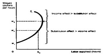
Now that we have some insight into the demand for labor, the next logical category is labor supply. We know that labor supply in competitive markets is highly elastic. But this fact does not answer two important questions: What determines the overall, or aggregate, supply of labor and how are wage rates and labor supply interrelated?

Individual Labor Supply

Individuals in free markets are able to choose whether to offer their labor services in the market, and individuals' labor market decisions are based on the principle of utility maximization. The individual must choose between time spent in the market earning the wage that he or she may command and time spent in nonmarket activities, such as going to school, keeping house, tending a garden, or watching television.

Fortunately, the individual does not have to make an all-or-nothing choice. No one chooses to work twenty-four hours a day, seven days a week. People can divide their time between market and nonmarket activities. How many hours would one choose to work during an average week? This question cannot be easily answered, but we can speculate about the effect that the wage rate may have on an individual's labor supply choices.

A supply curve relates the quantity supplied of a commodity to its price. Applied to labor supply, it is a schedule that relates the quantity of work offered and different wage rates. The labor supply curve of an individual is given in Figure 6.

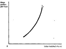
Figure 6. Individual Labor Supply

The individual labor supply curve, the number of hours offered at various wages, may be positively or negatively sloped. If the substitution effect is greater than the income effect, the curve is upward sloping, as shown from w, to w₃. The individual substitutes hours of work for hours of nonmarket activities. As the individual's wage rises beyond w₃, his or her demand for nonmarket time increases. The income effect is greater than the substitution effect, and the curve is negatively sloped above wage rate w₃.

Since the shapes of individual labor supply curves are difficult to determine, the slope of the total or aggregate labor supply curve is difficult to predict with accuracy. The aggregate labor supply curve is theoretically obtained by summing individuals' labor supply curves horizontally. The aggregate curve shows the total amount of labor supplied at all the different wages. Even though some individuals have backward-bending labor supply curves, we expect the aggregate labor supply curve to be positively sloped, in Figure 7, for two reasons. First, as wages rise, many workers will work more hours. Second, as wages rise, more people will enter the labor force.

Figure 7. The Aggregate Supply of Labor

The aggregate labor supply curve, S_A, representing the numbers of hours of labor supplied by all individuals, is likely to be upward sloping. As wages rise, more people join the labor force, and many people work more hours.

 

Although the wage rate has an influence on the number of hours people may choose to work, individuals may also choose their wage rate, within limits. They do so by choosing an occupation. Some occupations must pay higher wages than others to induce people to join.

Human capital: Any nontransferable quality an individual acquires that enhances productivity, such as education, experience, and skills.

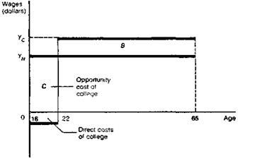
Figure 8. The Economic Costs and Benefits of College

An individual may choose to earn income Y_N from age eighteen to retirement at agesixty-five. Or an individual may attend college, lose income from age eighteen to age twenty-two, pay the direct costs of college, and then earn income Y_C from age twenty-two to retirement. The total costs of college are represented by the shaded area C, the lost income and direct costs; the benefits of college are shaded area B, the extra income earned with a college degree. In monetary terms it pays to go to college if B is greater than C.

Other Equalizing Differences in Wages

Total compensation: The lifetime income that an individual receives from employment in a particular occupation, including all monetary and nonmonetary pay.

Equalizing differences in wages: The differences in wages across all occupations that result in equality in total compensation.