Consumer Equilibrium: Diminishing Marginal Utility

Basic Assumptions

To use diminishing marginal utility to understand consumer behavior, four postulates of consumer behavior need to hold.

1. Each consumer desires a multitude of goods, and no one good is so precious that it will be consumed to the exclusion of other goods. Moreover, goods can be substituted for one another as alternative means of yielding satisfaction.

For example, the consumer good of exercise can be satisfied by jogging, playing basketball, hiking, swimming, or a number of other activities. Dinner offers a variety of choices—steak, chicken, pizza, and so on.

2. Consumers must pay prices for the things they want. This seems obvious, but for the purposes of the following analysis, it is important to assume that consumers face fixed prices for the things they consume.

3. Consumers cannot afford everything they want. They have a budget or income constraint that forces them to limit their consumption and to make choices about what they will consume.

4. Consumers seek the most satisfaction they can get from spending their limited funds for consumption. Consumers are not irrational. They make conscious, purposeful choices designed to increase their well-being. This does not mean that consumers do not make mistakes or sometimes make impulsive purchases that they later regret. But gaining experience over time as they deal in goods and services, consumers try to get the most possible satisfaction from their limited budgets given their past experience.

5. It is important to remember that only individuals make economic decisions. When we refer to a government agency, a corporation, or a snorkeling club as making a decision, we are only using a figure of speech. Take away the individual members who compose these organizations and nothing are left to make a decision. This reminder is a principle of positive economics, necessary' to avoid confusion.

6. Marginal utility analysis is an explanation, not a description, of individual choice behavior. Economists do not claim that individual consumers actually calculate marginal utility trade-offs before they go shopping. Indeed, most consumers, if asked, would probably deny that they behave in the way that marginal utility analysis suggests they do. The proof is obviously in the pudding. Individuals behave so as to generate the same outcomes they would generate if they actually did calculate and equate marginal utilities. Marginal utility analysis explains the outcomes we observe rather than describing the mental process involved.

Consumer equilibrium: A situation in which a consumer maximizes total utility within a budget constraint; equilibrium implies that the marginal utility obtained from the last dollar spent on each good is the same.

To express the general condition of consumer equilibrium, the equation given above is written with MU_x , MU_y, and so forth standing for the marginal utilities of different goods and P_x, P_y,and so forth representing the corresponding prices of the goods:

MU _{x =} MU _{y =} MU _{z =.} ...

P_x P_y P_z

 

From Diminishing Marginal Utility to the Law of Demand

 

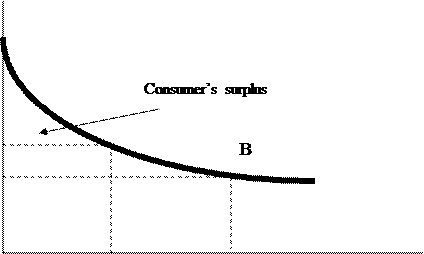
The law of demand says that consumers will respond to a fall in the relative price of a good by purchasing more of that good. Diminishing marginal utility thus provides a behavioral basis for the law of demand. When price falls, consumption increases until consumer equilibrium is again established.

The Substitution Effect and Income Effect

Substitution effect: The change in the quantity demanded of a particular good that results from a change in its price relative particular to other goods.

Real income: The buying power of money income; the quantities of goods and services that may be purchased with a given amount of dollar income.

Income effect: The change in quantity demanded of a particular good that results from a change in real income, which has resulted in turn from a change in price.

Consumers’ surplus (graph): The benefits that consumers receive from purchasing a particular quantity of a good at a particular price, measured by the area under the demand curve from the origin to the quantity purchased, minus price times quantity.

Price

A

 

P₁

P₀

 

Q₁ Q₀ Tomatoes purchased

Figure 3. Marginal Utility and Consumers' Surplus

 

Indifference Curve Analysis

 

Revealed preference: consumer's ordering of combinations of goods demonstrated through observations of the consumer s actions.

Indifference set: A group of combinations of two goods that yield the same total utility to a consumer.

Example: Suppose that four possible combinations of two goods confront an individual—say four possible combinations of quantities per week of vanilla and strawberry ice cream. Four combinations are given in Table 7.

Table 7

Combinations of Ice Cream Yielding Equal Total Utility

Combination	Scoops Per Week
Vanilla	Strawberry
A
B
C
D

 

Quantity scoops of vanilla per week

 

 

 

 

 

3 5 7 9 Quantity scoops of strawberry per week

Figure 4. An Indifference Curve

 

Indifference curve: A curve that shows all the possible combinations of two goods that yield the same total utility for a consumer.

Indifference curves have certain characteristics designed to show established regularities in the patterns of consumer preferences. Five of these characteristics are of interest to us.

1 Indifference curves slope downward from left to right. This negative slope is the only one possible if the principles of consumer choice are not to be violated. An upward-sloping curve would imply that the consumer was indifferent over the choice between a combination with less of both goods and another with more of both goods. The assumption that consumers always prefer more of a good to less requires that indifference curves slope downward from left to right.

2. The absolute value of the slope of the indifference curve at any point is equal to the ratio of the marginal utility of the good on the horizontal axis to the marginal utility of the good on the vertical axis.

Marginal rate of substitution: The amount of one good that an individual is willing to give up to obtain one more unit of another good.

3. Indifference curves are drawn to be convex: The slope of an indifference curve decreases as one move downward to the right along the curve. This convexity reflects diminishing marginal utility. As the quantity consumed of one of the goods increases, the marginal utility of that good declines.

4. A point representing any assortment of consumption alternatives will always be on some indifference curve.

Quantity eggs per week

 

 

 

 

1 4 5 8 9 Quantity strips of bacon per week

Figure 5. An Indifference Map

 

Indifference map: A graph that shows two or more indifference curves for a consumer.

5. Indifference curves, which are always drawn for only one individual over a given time period, never cross. The reason for this fact is called transitivity of preferences

Quantity eggs per week

 

 

 

5 6 8 Quantity strips of bacon per week

Figure 6. Indifference Curves Cannot Cross

Transitivity of preferences: A rational characteristic of consumers that suggests that if A is preferred to B and B is preferred to C, then A is preferred to C.

The Budget Constraint

Budget constraint: A line that shows all the possible combinations of two goods that an individual is able to purchase given a particular money income and price level for the two goods; budget line or consumption opportunity line.

The budget line is thus drawn to reflect any combination of prices for the two goods. The budget line is also called the consumption opportunity line because it shows the various combinations of goods that can be purchased at given prices with a given budget. The absolute value of the slope of the budget line is equal to the ratio of the price of the good on the horizontal axis to the price of the good on the vertical axis.

Apples per week (1$ per pound)

 

 

 

 

 

0 5 10 Oranges per week (1$ per pound)

(a) The budget line represents all possible combinations of apples and oranges at $1 per pound each within a budget constraint of $10 per week. The absolute value of the slope of the line is 1.

Apples per week (1$ per pound)

 

 

 

5 2

 

0 5 Oranges per week (1$ per pound)

(b) The budget line, still within the budget constraint of $10 per week, has changed to reflect an increase in the price of oranges to $2 per pound. The absolute value of the slope of the line is 2.

Figure 7. Budget Constraint