Kharkiv institute of banking

NATIONAL BANK OF UKRAINE

UNIVERSITY OF BANKING

KHARKIV INSTITUTE OF BANKING

 

MICROECONOMICS

Summary of Lectures

 

Composed by

Tatiana P. Bliznjuk

 

Kharkiv 2011

 

LECTURE 1: DEMAND AND SUPPLY

1. Individual and market demand

2. The elasticity of demand

3. Elasticity and total revenue

4. Cross elasticity of demand

5. Income elasticity of demand

6. Individual and market supply

7. Elasticity of supply

8. Supply elasticity and period

9. Review of supply and demand

Individual Demand and Market Demand

Demand is the schedule of quantities of a good or service that people purchase at different prices.

As the price of an item goes up, the quantity demanded falls, and as the price comes down, the quantity demanded rises. This inverse relationship may be stated as the law of demand.

Individual demand is the schedule of quantities that a person would purchase at different prices.

Market demand is the schedule of quantities that everyone in the market would buy at different prices.

Table 1

Hypothetical Individual Demand and Market Demand Schedules

Price	Quantity Demanded by
Ross	George	Bill	Ron	Total
$30

The Elasticity of Demand

Elasticity of demand measures the change in quantity in response to a change in price. We measure the responsiveness of quantity demanded to a change in price by calculating the coefficient of price elasticity of demand (E_p) as follows:

Percentage change in quantity demanded
Percentage change in price

If P1 is the initial price charged and P2 is the sale price, Q1 the initial quantity sold and Q2 the quantity sold during the sale, we can calculate the coefficient of price elasticity of demand as follows:

Percentage change in quantity demanded = Q₁ - Q ₂ x P₁+ P₂
Percentage change in price Q₁ + Q₂ P₁ - P₂

Example: A business firm had been selling 100 kitchen chairs a week. It runs a sale, charging $8 instead of the usual $10. People recognize this great bargain, and sales go up to 140 chairs.

Solution: P₁ = 10; P₂ = 8; Q₁ = 100; and Q₂= 140.

140-100 x 10+8 = 40 x 18 = 4 x 9 = 1 x 9 = 9 = 3

100+140 8-10 240 -2 24 1 6 1 6 2

Elasticity is the percentage change in quantity demanded brought about by a price change. In essence, it is percentage change in quantity divided by percentage change in price.

The border between elastic and inelastic is one. If elasticity is less than one, it is inelastic. If it is exactly one, it is unit elastic. If elasticity is more than one, it is elastic.

In Figure 1 we have aperfectly elastic demand curve. It is horizontal. Perfect elasticity is ¥.

In Figure 2 we have a perfectly inelastic demand curve. Perfect elasticity is 0. It is vertical line.

 

 

Figure 1. Perfectly elastic demand curve

 

 

Figure 2. Perfectly inelastic demand curve

Figure 3 show us relative elasticity.

 

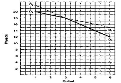
Figure 3. Relative elasticity

D₁ is more elastic because it is closer to being horizontal. The more horizontal the demand curve is, the more elastic it is, and the more vertical the curve, the more inelastic it is.

Unit elasticity means that when a price change causes quantity demanded to change by the same percentage.

A straight line demand curve that moves downward to the right is very elastic at the top and progressively less elastic as we move down the curve.

 

 

 

Figure 4.

 

Elasticity and Total Revenue

Total revenue = Price x Quantity

When demand is elastic, if we were to raise price, total revenue would fall.

When demand is elastic, if we were to lower price, total revenue would rise.

When demand is inelastic, if we were to raise price, total revenue would rise.

When demand is inelastic and price is lowered, total revenue will fall.

 

Cross Elasticity of Demand

 

We calculate the coefficient of cross elasticity of demand E_xy just as we do the coefficient of simple price elasticity, except that we relate the percentage change in the consumption of product X to the percentage change in the price of product Y:

E_xy = percentage change in quantity demanded of product X

percentage change in price of product Y

This cross elasticity concept allows us to quantify and more fully understand substitute and complementary goods.

Substitute Goods. If cross elasticity of demand is positive—that is, the quantity demanded of X moves in the same direction as a change in the price of Y— then X and Y are substitute goods.

Complementary Goods. When cross elasticity is negative, we know that X and Y "go together"; an increase in the price of one decreases the demand for the other. So these two are complementary goods.

Independent Goods. A zero or near-zero cross elasticity suggests that the two products are unrelated or independent goods.

 

Income Elasticity of Demand

 

Income elasticity of demand measures the degree to which consumers respond to a change in their incomesby buying more or less of a particular good. The coefficient of income elasticity of demand E_i is determined with the formula:

E_i = percentage change in quantity demanded

percentage change in income

Normal Goods. For most goods the income elasticity coefficient E_i is positive, meaning that more of them is demanded as incomes increase. Such goods are called normal or superior goods. But the value of E_i varies greatly among normal goods.

Inferior Goods. A negative income elasticity coefficient designates an inferior good. Retreaded tires, cabbage, long-distance bus tickets, used clothing, and muscatel wine are likely candidates. Consumers decrease their purchases of such products as incomes increase.

Insights. Income elasticity of demand coefficients provides insights about the economy.

Table 2

Cross and income elasticities of demand

Value of coefficient	Description	Type of good(s)
Cross elasticity: Positive (Ewz>0)     Negative (Ewz<0)	Quantity demanded of W changes in same direction as change in price of Z   Quantity demanded of X changes in opposite direction from change in price of Y	Substitutes     Complements
Income elasticity: Positive (Ei > 0)     Negative (Ei < 0)	Quantity demanded of the product changes in same direction as change in income   Quantity demanded of the product changes in opposite direction from change in income	Normal or superior     Inferior

 

Elasticity of supply

Percentage change in quantity supplied = Q₁ - Q ₂ x P₁+ P₂
Percentage change in price Q₁ + Q₂ P₁ - P₂

Figure 6 shows a perfectly elastic supply curve, which is exactly the same as a perfectly elastic demand curve.

Figure 7 shows a perfectly inelastic supply curve, which would be identical to a perfectly inelastic demand curve.

 

Figure 6. Perfectly elastic supply curve

 

Figure 7.Perfectly inelastic supply curve

Figure 8 shows relative elasticity of supply.

Figure 8. Relative elasticity of supply

 

Average Cost

Average fixed cost (AFC) = Fixed cost/Output

Average variable cost (AVC) = Variable cost/Output

Average total cost (ATC) = Total cost / Output.

Table 3

Hypothetical Cost Schedule

Output	Variable Cost	Total Cost	AFC	AVC	ATC	Marginal Cost
	$100	$ 500	$400	$100	$500	$100
		1,000
		1,219

Figure 10. Graphing the AFC, AVC, ATC, and MC Curves

Revenue and Profit

Table 4

Hypothetical Revenue Schedule

Output	Price	Total Revenue	Marginal Revenue
	$5	$ 5	$5

Figure 11.

9. Review of Supply and Demand

 

 

Figure 12. Market equilibrium

We also analyzed changes in demand and changes in supply.

Example: Find the new equilibrium price and quantity in Figure 13.

Solution: The new equilibrium price is $8.0 and the new equilibrium quantity is 70.

 

 

Figure 13. An increase in demand

Utility

 

Utility isthe ability of a good to satisfy wants; the satisfaction obtained from the consumption of goods.

Principle of diminishing marginal utility: As people consume a good in greater and greater quantities, eventually they get less and less extra utility from further increases in consumption.

Marginal utility is the additional utility derived from consuming one more unit of some good or service.

Table 1

Hypothetical Demand Schedule for Hamburgers

Price	Quantity Demanded
$2.75
2.00
1.00
.25

Marginal utility: The change in total utility that results from the consumption of one more unit of a good; the change in total utility divided by the change in quantity consumed.

Table 2

Total Utility and Marginal Utility

Scoops of ice cream	Total utility Marginal utility (utils) (extra utils per scoop)
	6 6 11 5 15 4 18 3 20 2

Total utility is the utility you derive from consuming a certain number of units of a good or service. To get total utility, just add up the marginal utilities of all the units purchased. We've done that in Table 3.

Table 3

Hypothetical Utility Schedules

Units Purchased	Marginal Utility	Total Utility
	$2.75	$2.75
	2.00	4.75
	1.00	5.75
	.25	6.00

Total utility: The total amount of satisfaction obtained from the consumption of a particular quantity of a good, a summation of the marginal utility obtained from consuming each unit of a good.

 

Total

utility

 

0 1 2 3 4 5

(a) Total utility

Marginal

utility

 

0 1 2 3 4 5

(b) Marginal utility

Figure 1. Total Utility and Marginal Utility

(a) Total utility increases at a decreasing rate as more and more ice cream is consumed in one sitting.

(b) Marginal utility declines with each additional scoop of ice cream at one sitting.

 

Since we buy a good or service up to the point at which its marginal utility is equal to its price, we could form this simple equation:

Marginal utility

Price

We keep buying a good until itsMU declines to the price level. In fact, the same thing can be said about everything we buy. To generalize,

MU₁ = MU₂ = MU₃ = MU_n

P₁ P₂ P₃ P_n

Example: You are ravenously hungry, so you decide to do lunch. You're going to try something a little different this time—hamburgers, french fries, and a coke or two.

Table 4

Your Demand and Marginal Utility

Schedules for Hamburgers

Price	Quantity demanded	Marginal utility
$3		$3

 

Table 5

Your Demand and Marginal Utility

Schedules for French Fries

Price	Quantity demanded	Marginal utility
$1.50		$1.50
1.00
0.50		0.50

Table 6

Your Demand and Marginal Utility

Schedules for Cokes

Price	Quantity demanded	Marginal utility
$1.50		$1.50
0.50		0.50

Now let's put all these numbers into our formula:

MU₁ = MU₂ = MU₃

P₁ P₂ P₃

I'd like you to substitute the marginal utilities and prices of (1) hamburgers, (2) french fries, and (3) cokes:

$3 = $0.50 = $0.50

$3 $0.50 $0.50

Let's see how many burgers, fries, and cokes you'd chow down if burgers were $1, fries were $1, and Cokes were $1.50. You would have purchased three burgers, two fries, and one coke.

Now set up your MU/Price equation, substituting your fingers for burgers, fries, and cokes.

$1 = $1 = $1.50

$1 $1 $1.50

Why did you shift from one burger to three? Because their price came down. And why did you buy fewer fries and cokes? Because their prices rose. Now we come to that elusive point we've been trying to make. We're always maximizing our utility. We'll buy more and more of a particular good or service until its MU declines to its price (remember our law of diminishing marginal utility).

You maximized your utility by purchasing one hamburger when its price was $3, three fries at $0.50 each, and two cokes at $0.50 each. But when the price of hamburgers fell to $1, you bought three. And you bought just two orders of fries when their price rose to $1 and just one Coke at $1.50.

 

Consumer Surplus

Consumer surplus is the difference between what you pay for some good or service and what you would have been willing to pay.Usually, when you buy something, you actually would have been willing to pay even more.

Example: If the price of hamburgers were a quarter, four would be purchased and the consumer surplus would be the triangular area above the price line in Figure 2. The total consumer surplus would be based on the difference between what you paid for each hamburger (25 cents) and what you would have been willing to pay. You would have been willing to pay $2.75 for the first one, so your consumer surplus on the first hamburger is $2.50. You would have been willing to pay $2 for the second, so on that one your consumer surplus is $1.75. Similarly, on the third hamburger your consumer surplus is $1.00 - 0.25 = $0.75. On the fourth hamburger, since MU = Price (25 cents = 25 cents), there is no consumer surplus. Your total consumer surplus would be $2.50 + $1.75 + $.75 = $5. Looked at another way, your total utility derived from the four hamburgers is $6 and if you pay 25 cents for each four hamburgers, $6 minus $1 equals a consumer surplus of $5.

No one ever paid more than he or she was willing to pay; no one ever bought anything whose price exceeded its utility; and anyone who ever bought several units of the same product at a fixed price enjoyed a consumer surplus.

 

 

 

0.25

1 2 3 4

 

Figure 2. Consumer surplus

 

Basic Assumptions

To use diminishing marginal utility to understand consumer behavior, four postulates of consumer behavior need to hold.

1. Each consumer desires a multitude of goods, and no one good is so precious that it will be consumed to the exclusion of other goods. Moreover, goods can be substituted for one another as alternative means of yielding satisfaction.

For example, the consumer good of exercise can be satisfied by jogging, playing basketball, hiking, swimming, or a number of other activities. Dinner offers a variety of choices—steak, chicken, pizza, and so on.

2. Consumers must pay prices for the things they want. This seems obvious, but for the purposes of the following analysis, it is important to assume that consumers face fixed prices for the things they consume.

3. Consumers cannot afford everything they want. They have a budget or income constraint that forces them to limit their consumption and to make choices about what they will consume.

4. Consumers seek the most satisfaction they can get from spending their limited funds for consumption. Consumers are not irrational. They make conscious, purposeful choices designed to increase their well-being. This does not mean that consumers do not make mistakes or sometimes make impulsive purchases that they later regret. But gaining experience over time as they deal in goods and services, consumers try to get the most possible satisfaction from their limited budgets given their past experience.

5. It is important to remember that only individuals make economic decisions. When we refer to a government agency, a corporation, or a snorkeling club as making a decision, we are only using a figure of speech. Take away the individual members who compose these organizations and nothing are left to make a decision. This reminder is a principle of positive economics, necessary' to avoid confusion.

6. Marginal utility analysis is an explanation, not a description, of individual choice behavior. Economists do not claim that individual consumers actually calculate marginal utility trade-offs before they go shopping. Indeed, most consumers, if asked, would probably deny that they behave in the way that marginal utility analysis suggests they do. The proof is obviously in the pudding. Individuals behave so as to generate the same outcomes they would generate if they actually did calculate and equate marginal utilities. Marginal utility analysis explains the outcomes we observe rather than describing the mental process involved.

Consumer equilibrium: A situation in which a consumer maximizes total utility within a budget constraint; equilibrium implies that the marginal utility obtained from the last dollar spent on each good is the same.

To express the general condition of consumer equilibrium, the equation given above is written with MU_x , MU_y, and so forth standing for the marginal utilities of different goods and P_x, P_y,and so forth representing the corresponding prices of the goods:

MU _{x =} MU _{y =} MU _{z =.} ...

P_x P_y P_z

 

Indifference Curve Analysis

 

Revealed preference: consumer's ordering of combinations of goods demonstrated through observations of the consumer s actions.

Indifference set: A group of combinations of two goods that yield the same total utility to a consumer.

Example: Suppose that four possible combinations of two goods confront an individual—say four possible combinations of quantities per week of vanilla and strawberry ice cream. Four combinations are given in Table 7.

Table 7

Combinations of Ice Cream Yielding Equal Total Utility

Combination	Scoops Per Week
Vanilla	Strawberry
A
B
C
D

 

Quantity scoops of vanilla per week

 

 

 

 

 

3 5 7 9 Quantity scoops of strawberry per week

Figure 4. An Indifference Curve

 

Indifference curve: A curve that shows all the possible combinations of two goods that yield the same total utility for a consumer.

Indifference curves have certain characteristics designed to show established regularities in the patterns of consumer preferences. Five of these characteristics are of interest to us.

1 Indifference curves slope downward from left to right. This negative slope is the only one possible if the principles of consumer choice are not to be violated. An upward-sloping curve would imply that the consumer was indifferent over the choice between a combination with less of both goods and another with more of both goods. The assumption that consumers always prefer more of a good to less requires that indifference curves slope downward from left to right.

2. The absolute value of the slope of the indifference curve at any point is equal to the ratio of the marginal utility of the good on the horizontal axis to the marginal utility of the good on the vertical axis.

Marginal rate of substitution: The amount of one good that an individual is willing to give up to obtain one more unit of another good.

3. Indifference curves are drawn to be convex: The slope of an indifference curve decreases as one move downward to the right along the curve. This convexity reflects diminishing marginal utility. As the quantity consumed of one of the goods increases, the marginal utility of that good declines.

4. A point representing any assortment of consumption alternatives will always be on some indifference curve.

Quantity eggs per week

 

 

 

 

1 4 5 8 9 Quantity strips of bacon per week

Figure 5. An Indifference Map

 

Indifference map: A graph that shows two or more indifference curves for a consumer.

5. Indifference curves, which are always drawn for only one individual over a given time period, never cross. The reason for this fact is called transitivity of preferences

Quantity eggs per week

 

 

 

5 6 8 Quantity strips of bacon per week

Figure 6. Indifference Curves Cannot Cross

Transitivity of preferences: A rational characteristic of consumers that suggests that if A is preferred to B and B is preferred to C, then A is preferred to C.

The Budget Constraint

Budget constraint: A line that shows all the possible combinations of two goods that an individual is able to purchase given a particular money income and price level for the two goods; budget line or consumption opportunity line.

The budget line is thus drawn to reflect any combination of prices for the two goods. The budget line is also called the consumption opportunity line because it shows the various combinations of goods that can be purchased at given prices with a given budget. The absolute value of the slope of the budget line is equal to the ratio of the price of the good on the horizontal axis to the price of the good on the vertical axis.

Apples per week (1$ per pound)

 

 

 

 

 

0 5 10 Oranges per week (1$ per pound)

(a) The budget line represents all possible combinations of apples and oranges at $1 per pound each within a budget constraint of $10 per week. The absolute value of the slope of the line is 1.

Apples per week (1$ per pound)

 

 

 

5 2

 

0 5 Oranges per week (1$ per pound)

(b) The budget line, still within the budget constraint of $10 per week, has changed to reflect an increase in the price of oranges to $2 per pound. The absolute value of the slope of the line is 2.

Figure 7. Budget Constraint

 

No influence.

- If any action taken by the firm has any effect on price, that's influence.

- If a firm, by withholding half its output from the market was able to push up price, that would be influence.

- If a firm doubled its output and forced down price, that too would be influence.

- If a firm left the industry, which would make price go up, that would be influence on price.

Number of firms.

The industry under perfect competition includes many firms. So many that no one firm has any influence on price.

3. The perfect competitor is a price taker rather than a price maker. Price is set by industry wide supply and demand; the perfect competitor can take it or leave it.

Product.

For perfect competition to take place, all the firms in the industry must sell an identical, or standardized, product. That is, those who buy the product cannot distinguish between what one seller and another sells. So, in the buyer's mind, the product is identical. The buyer has no reason to prefer one seller to another.

A perfectly competitive industry has many firms selling an identical product. How many is many? So many that no one firm can influence price. What is identical? A product that is identical in the minds of buyers so that they have no reason to prefer one seller to another.

We've already discussed the two most important characteristics—actually, requirements—of perfect competition: many firms and an identical product. Two additional characteristics are perfect mobility and perfect knowledge.

 

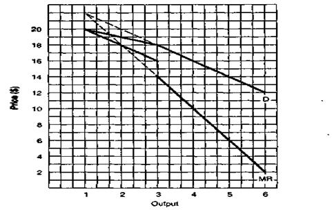
The Short Run

In the short run, the perfect competitor may make a profit or lose money.

In the long run, as we'll see, the perfect competitor just breaks even.

Figure 2 shows one example of a perfect competitor in the short run.

Price Price

MR

D

The Long Run

In the long run, there is time for firms to enter or leave the industry. This factor ensures that the firm will make zero profits in the long run. What was an unlikely outcome for the firm in the short run—zero profits—becomes an absolute certainty in the long run.

If one firm is losing money, presumably others are too; given the extent of the short-run losses this individual firm is suffering, chances are other firms too are ready to go out of business.

Example: When enough firms go out of business, industry supply declines from S₁ to S₂, which pushes price up from $6 to $8. This price rise is reflected in a new demand curve for the firm in the left side of Figure 6. In short, a decline in industry supply from S, to S₂ pushes up the firm's demand curve from D₁ to D₂.

Figure 6. A perfect competitor in long run

If one firm is making a profit, we can assume others are too. New firms will spring up, and entrepreneurs will enter the industry to get their share of the profits. As more and more firms enter the industry, market supply increases, pushing the supply curve to the right (on the right side of Figure 7).

Figure 7. A perfect competitor in long run

The left side of Figure 6 and the left side of Figure 7 are identical. Notice that the ATC and the demand/MR curves is tangent (just touching). At that point of tangency, MC equals MR, so that is where the firm produces. ATC equals price at that point, so profit is zero.

Example: Figure 8 shows the firm'sdemand and MR curve just tangent (or touching) the ATC curve. The price is$18.50, and the output is 11.

Figure 8.A perfect competitor in long run

Efficiency

For the perfect competitor in the long run, the most profitable output is at the minimum point of its ATC curve. At any other output, the firm would lose money; just to stay in business; it must operate at peak efficiency.

This is the hallmark of perfect competition. The firm, not through any virtues of its owners but because of the degree of competition in the marketplace, is forced to operate at peak efficiency. The other forms of competition do not force peak efficiency.

Competition is very good for the consumer. She or he can buy at cost. That's right, price is equal to ATC. Remember—no economic profit. And consumers have the firm's competitors to thank for such a low price. Competition will keep business owners honest—that is, if there's enough competition.

 

Definition of Monopoly

 

There's nobody else selling anything like what the monopolist is producing. In other words, there are no close substitutes.

The Graph of the Monopolist

 

Monopoly is the first of three types of imperfect competition. The distinguishing characteristic of imperfect competition is that the firm's demand curve is no longer a perfectly elastic horizontal line; now it curves downward to the right. This means the imperfect competitor will have to lower price to sell more.

Table 1

Hypothetical Demand and Cost Schedule for a Monopoly

Output	Price	Total Revenue	Marginal Revenue	Total Cost	ATC	MC
	$16	$16	$16	$20	$20	-
						$10
					10.50
					10.50

MC is the additional cost of producing one more unit of output. As output rises, fixed cost stays the same and variable cost rises.

MC of the first unit of output would be total cost at output 1 minus total cost at output zero.

The ATC and MC curves are the same as they were for the perfect competitor. The demand and marginal revenue curves slope downward to the right.

Example: At 1 unit of output, the demand and marginal revenue curves share the same point—$16—but the MR curve then slopes down much faster. In fact, when the demand curve is a straight line, the marginal revenue curve is also a straight line that falls twice as quickly.

Figure 1. Monopoly

 

If the seller lowers price to sell more output, the price is lowered on all units of output, not just on the last one. This is what drives down MR faster than price (which is read off the demand curve).

 

How to Read a Graph

Example: Our output is always determined by the intersection of the MC and MR curves. That occurs at an output of about 4.25.

How much is price? First, price is read off the demand curve. Where on the demand curve—at what output? At the maximum profit output we just found—4.25. How much is price at that output? It appears to be about $9.

Next we calculate total profits.

Total profits = (Price - ATC)xOutput = ($9 - $7.50) x 4.25=$1.50x4.25= $6.38

You might have noticed that once we find output (where MC = MR), everything else lines up. Price is located on the demand curve above the output of 4.25. ATC is on the ATC curve, also above an output of 4.25. When we find total profits, we plug price, ATC, and output into our formula.

Figure 2. Monopoly

Microeconomics is based largely on the three-step problems you've come to know: (1) filling in the table, (2) drawing the graph, and (3) doing the analysis.

We need to find the monopolist's total profit. Do that right here. Then check your work with the calculations that follow.

Total profit = (Price - ATC) x Output = ($17 - $14) x 5 = $3x5 = $15

Table 2

Hypothetical Demand and Cost Schedule for a Monopoly

Output	Price	Total Revenue	Marginal Revenue	Total Cost	ATC	MC
	$21	$21	$21	$30	$30	-
						$10
					14.25
					15.50

 

Analyze:

1. At what output would the firm produce most efficiently?

2. At what output would the perfect competitor produce in the long run?

3. What price would the perfect competitor charge in the long run?

Here are the answers.

1. The output at which the firm would produce most efficiently would be about
5.1, which is the minimum point of the ATC curve.

2. The perfect competitor would produce at an output of 5.1 in the long run.

3. In the long run, the perfect competitor would charge a price of about $13.97 (the minimum, or break-even, point of the ATC curve).

 

Barriers to Entry

 

There are three barriers to entry: (1) control over an essential resource, (2) economies of scale, and (3) legal barriers to entry.

Figure 2. Hypothetical Production Costs for Cars

In some industries, low unit costs may be achieved only through large-scale production. Such economies of scale put potential entrants at a disadvantage. To be able to compete effectively in the industry, a new firm has to enter on a large scale, which can be costly and risky. The effect is to deter entry. Only rarely do new firms attempt to enter the automobile manufacturing industry, for example, because it uses highly automated production techniques on a large scale to keep costs down.

Natural monopoly: A monopoly that occurs because of a particular relation between industry demand and the firm's average total costs that makes it possible for only one firm to survive in the industry.

Legal barriers: legal franchise, license, or patent granted by government that prohibits other firms or individuals from producing particular products or entering particular occupations or industries.

The whole idea is for the government to allow just one firm or a group of individuals to do business.

First, it may be necessary to obtain a public franchise to operate in an industry.

Second, in many industries and occupations a government license is required to operate.

Public franchise: A right granted to a firm or industry allowing it to provide a good or service and excluding competitors from providing that good or service.

Government license: A right granted by state or federal government to enter certain occupations or industries.

Patent: A monopoly granted by government to an inventor for a product or process.

LECTURE 5: MONOPOLISTIC COMPETITION

1. Monopolistic Competition Definition

2. The monopolistic competitor in the short and long runs

3. Product differentiation

4. Price discrimination

 

To sum up, both the monopolistic competitor and the perfect competitor make zero economic profits in the long run. The monopolistic competitor charges a higher price and has a lower output than the perfect competitor and the perfect competitor is a more efficient producer than the monopolistic competitor.

 

Product Differentiation

 

Product differentiation is crucial to monopolistic competition. In fact, product differentiation is really what stands between perfect competition and the real world. People differentiate among many similar products.

What makes one good or service differ from another? We need only for the buyer to believe it's different, because product differentiation takes place in the buyer's mind. In the real world, however, buyers generally do differentiate. We're always differentiating, and it doesn't have to be based on taste, smell, size, or even any physical differences among the products.

The monopolistic competitor faces a more elastic, or flatter, demand curve than the monopolist.

 

 

Figure 4. The Typical Monopolistic Competitor

 

Price Discrimination

 

Price discrimination occurs when a seller charges two or more prices for the same good or service.

The most notorious example of price discrimination was probably that of A&P during the 1940s. A&P had three grades of canned goods: A, B, and C. Grade A was presumably of the highest quality, B was fairly good, and C was— well, C was edible. My mother told me that she always bought grade A, even though it was the most expensive. Nothing but the best for our family. Our family was friendly with another family in the neighborhood. The husband, a man in his early 50s, found out he had stomach cancer. "Aha!" exclaimed my mother, "Mrs. S. always bought grade C!"

A few years later the Federal Trade Commission (FTC) prohibited A&P from selling grades A, B, and C. The FTC didn't do that because of Mr. S.'s stomach cancer, but because there was absolutely no difference among the grades.

Why had A&P concocted this elaborate subterfuge? Because it was worth tens of millions of dollars in profits! Take a can of green peas that had a demand schedule like the one in Table 1.

To keep things simple, suppose A&P had a constant ATC of 20 cents a can. How much should it charge? To figure this out, add a total cost column to Table 1 and then a total profits column. Now figure out the total profits at prices of 50 cents, 40 cents, and 30 cents, respectively.

In Table 2, these calculations are all worked out. If A&P could charge only one price, it would be 50 cents; total profit would be $30. Now let's see how much profit would be if A&P were able to charge three different prices.

 

Table 1

Hypothetical Demand Schedule for Canned Peas

Price	Quantity Demanded	Total Revenue
$ 0.50		$50
0.40
0.30

At 50 cents, A&P would be able to sell 100 cans. These are sold to the people who won't buy anything if it isn't grade A. Then there are those who would like to buy grade A but just can't afford it. These people buy 40 cans of grade B. Finally, we have the poor, who can afford only grade C; they buy 30 cans.

Table 2

Hypothetical Demand Schedule for Canned Peas

Price	Total Revenue	Total Cost	Total Profit
$ 0.50	$50	$20	$30
0.40
0.30

All this is worked out in Table 3. Total revenue now is $75 for the 170 cans sold, and total cost of 170 cans remains $34. This gives A&P a total profit of $41.

Table 3

Hypothetical Demand Schedule for Canned Peas, by Grades

Grade	Price	Quantity Demanded	Total Revenue	Total Costs	Total Profit
A	$ 0.50		$50	$20	$30
B	0.40
C	0.30
Sum			$75	$34	$41

Why is total profit so much greater under price discrimination ($41) than it is under a single price ($30)? Total profit would be $30 at 50 cents; it would be $28 at 40 cents; it would be $17 at 30cents. Because the seller is able to capture some or all of the consumer's surplus. People are willing to buy only 100 cans at 50 cents, 40 more at 40 cents, and another 30 at 30 cents. But the people who buy only grade A will buy all their cans of green peas at that price, while those buying grade B will buy all their peas at 40 cents and grade C buyers will buy all their peas at 30 cents. By keeping its markets separate rather than charging a single price, A&P had been able to make much larger profits.

The firm that practices price discrimination needs to be able to distinguish between two or more separate groups of buyers.

In addition to distinguishing among separate groups of buyers, the price discriminator must be able to prevent buyers from reselling the product (i.e., stop those who buy at a low price from selling to those who would otherwise buy at a higher price).

Monopolistic competitors do compete with respect to price, but they compete still more vigorously with respect to ambience, service, and the rest of the intangibles that go along with attracting customers. To the degree that they're successful, they have gotten you to differentiate their product from all the others. That is what monopolistic competition is all about.

LECTURE 6: OLIGOPOLY

1.Oligopoly Definition

2.Concentration ratios

3.The competitive spectrum

4.The kinked demand curve

5.Administered prices

 

Oligopoly Definition

An oligopoly is an industry with just a few sellers. The crucial factor under oligopoly is the small number of firms in the industry. Because there are so few firms, every competitor must think continually about the actions of his rivals, since what each does could make or break him. Thus there is a kind of interdependence among oligopolists.

Because the graph of the oligopolist is similar to that of the monopolist, we will analyze it in exactly the same manner with respect to price, output, profit, and efficiency. Price is higher than the minimum point of the ATC curve, and output is somewhat to the left of this point. And so, just like the monopolist, the oligopolist has a higher price and a lower output than the perfect competitor.

The oligopolist, like the monopolist and unlike the perfect competitor, makes a profit. With respect to efficiency, since the oligopolist does not produce at the minimum point of its ATC, it is not as efficient as the perfect competitor.

Concentration ratios

One way of measuring how concentrated an industry is, is to look at the percentage share of sales of the leading firms. This is called the industry's concentration ratio.

Economists use concentration ratios as a quantitative measure of oligopoly. The total percentage share of industry sales of the four leading firms is the industry concentration ratio. Industries with high ratios are very oligopolistic.

Two key shortcomings of concentration ratios should be noted.

1. They don't include imports.

2. The concentration ratios tell us nothing about the competitive structure of the rest of the industry.

A second way is to calculate the Herfindahl-Hirschman index, which, it turns out, is a lot easier to do than to say.

The Herfindahl-Hirschman Index (HHI). The Herfindahl-Hirschman index (HHI) is the sum of the squares of the market shares of each firm in the industry.

Find the HHI of an industry with just two firms, both of which have 50 percent market shares. Work it out right here:

50² + 50² = 2,500 + 2,500 = 5,000

 

The Competitive Spectrum

 

Cartel

An extreme case of oligopoly is a cartel, where the firms behave as a monopoly in a manner similar to that of the Organization of Petroleum Exporting Countries (OPEC) in the world oil market.

Figure 1. Cartel

Open Collusion.

Slightly less extreme than a cartel would be a territorial division of the market among the firms in the industry. This would be a division similar to that of the Mafia, if indeed there really is such an organization. An oligopolistic division of the market might go something like this.

Figure 2. The Colluding Oligopolist

 

 

Figure 3. The Competitive Spectrum

The Kinked Demand Curve

 

Now we deal with the extreme case of oligopolists who are cutthroat competitors, firms that do not exchange so much as a knowing wink. Each is out to maximize its profits. These oligopolists are ready to cut the throats of their competitors, figuratively speaking, of course.

The uniqueness of this situation leads us to the phenomenon of the kinked demand curve, pictured in Figure 4. For the first time in this course, we have a firm's demand curve that is not a straight line.

Figure 4. The kinked demand curve

Let's examine the kinked demand curve a little more closely. It's really two demand curves in one, the left segment being relatively elastic (or horizontal) and the right less elastic (more vertical).

In Figure 5, both segments of the demand curve have been extended. This was done to set up the next step, the MR curves of Figure 6. Before we can figure out the oligopolist's actual MR curve, we'll have to see how each of the MR curves in Figure. 6 is drawn.

Figure 5

Figure 6

 

Figure 7

Using the data from Table 1, draw the firm's demand and MR curves. A very tricky part comes when we do the MR curve at its discontinuity (when it drops straight down). This part always lies directly below the kink in the demand curve.

Table 1

Hypothetical Demand Schedule for Competing Oligopolist

Output	Price	Total Revenue	Marginal Revenue
	$50	$50	$50

Figure 8

How much are output, price, and total profit (table 2, figure 9)? Output, which is directly under the kink, is 4. Price, which is at the kink, is$27. Remember that price is always read off the demand curve. And now, total profit:

Total profit = (Price - ATC) x Output= ($27 - $24) x 4 = $3x4 = $12

Table 2

Hypothetical Demand and Cost Schedule for Competitive Oligopolist

Output	Price	Total Revenue	Marginal Revenue	Total Cost	ATC	Marginal Cost
	$30	$30	$30	$40	$40	-
						$20

Figure 9

Can you come up with an easier way of finding the firm’s total profit? Look at Table 2 again. Just subtract total cost from total revenue at an output of 4 ($108 — $96 = $12). Once you know the output, all you need to do is subtract TC from TR.

 

Administered Prices

 

Administered prices are set by large corporations for relatively long periods of time, without responding to the normal market forces, mainly, changes in demand.

Summary

LECTURE 7: THE FIRM

1. Market and Firm Coordination

2. Size and Types of Business Organizations

3. The Balance Sheet of a Firm

 

Scale of Production

As we have seen, firms evolve when team effort can produce goods and services at a lower cost than individual effort. This occurs because of the increased efficiency that may be gained when labor and capital are coordinated through managerial talents. In the following sections, we consider the varying sizes of firms and the advantages and disadvantages of various ways that firms can be organized.

The most efficient size for firms (the size that performs at the lowest cost of production) varies greatly. The most efficient scale of production can be as small as a hot dog stand on a street comer or as large as a General Motors assembly plant.

Scale of production: The relative size and rate of output of a physical plant that may be measured by the volume or value of firm capital.

Categories of Ownership

Generally, a firm is organized to fit one of three legal categories:

1) proprietorship;

2) partnership;

3) corporation.

The nature of ownership is different in each category.

 

Proprietorship

Proprietorship: Is a firm that has a single owner who is liable — or legally responsible — for all the debts of the firm, a condition termed unlimited liability. The sole proprietor has unlimited liability in the legal sense that if the firm goes bankrupt, the proprietor's personal as well as business property can be used to settle the firm's outstanding debts.

Unlimited liability: A legal term that indicates that the owner or owners of a firm are personally responsible for the debts of a firm up to the total value of their wealth.

More often than not, the sole proprietor also works in the firm as a manager and a laborer. Obviously, most single-owner firms are small. Many small retail establishments are organized as proprietorships.

The primary advantage of the proprietorship is that it allows the small businessperson direct control of the firm and its activities. The owner, who is the residual claimant of profits over and above all wage payments and other expenses, monitors his or her own performance. The sole proprietor faces a market price directly. It is up to the sole proprietor to decide how much effort to expend in producing output. In other words, the sole proprietor can be his or her own boss.

The primary disadvantage of the proprietorship is that the welfare of the firm largely rests on one person. The typical sole proprietor is the chief stockholder, chief executive officer, and chief bottle washer for the firm. Since there are only twenty-four hours in a day, the sole proprietor faces problems in attending to the various aspects of the business.

 

Partnership

Partnership: Is an extended form of the proprietorship. Rather than one owner, a partnership has two or more co-owners. These partners — who are team members — share financing of capital investments and, in return, the firm's residual claims to profits. Jointly they perform the managerial function within the firm, organizing team production and monitoring one another's behavior to control shirking. A partnership is a form well suited to lines of team production that involve creative or intellectual skills, an area in which monitoring is difficult. Imagine trying to direct a commercial artist's work in detail or monitoring a lawyer's preparation for a case.

The partnership also has certain limitations. Individual partners cannot sell their share of the partnership without the approval of the other partners. The partnership is terminated each time a partner dies or sells out, resulting in costly reorganization. And each partner is considered legally liable for all the debts incurred by the partnership up to the full extent of the individual partner's wealth, a condition called joint unlimited liability. Because of these limitations, partnerships are usually small and are found in businesses where monitoring of production by a manager is difficult.

Joint unlimited liability: The unlimited liability condition in a partnership that is shared by all partners.

 

Corporation

While corporations are not the most numerous form of business organization, they conduct most of the business. This means that many large firms are corporations and that this form of business organization must possess certain advantages over the proprietorship and the partnership in conducting large-scale production and marketing.

In a corporation, ownership is divided into equal parts called shares of stock. If any stockholder dies or sells out to a new owner, the existence of the business organization is not terminated or endangered as it is in a proprietorship or partnership. For this reason the corporation is said to possess the feature of continuity.

Share: The equal portions into which the ownership of a corporation is divided.