Economic Profits Versus Accounting Profits

Businesspeople must compare their total costs with their total revenues (all the money they take in) to determine whether they are making a profit.

Economic profit is the difference between total revenue and total cost. It exists when the revenue of the firm more than covers all of its costs, explicit and implicit. Economic loss results when revenue does not cover the total cost. A firm's economic profit is said to be zero when its total revenue equals its total cost.

Zero economic profit does not mean that the firm is not viable or about to cease operating. It means that the firm is covering all the costs of its operations and that the owners and investors are making a normal rate of return on their investment.

Since accounting costs do not usually include implicit costs — such as the value of the sole proprietor's time or the opportunity cost of capital invested in the firm — accounting costs are an understatement of the opportunity costs of production. This means that accounting profits will generally be higher than economic profits because economic profits are calculated after taking both explicit and implicit costs into account.

Private costs: The total opportunity costs of production for which the owner of a firm is liable.

External costs: The costs of a firm's operation that it does not pay for.

Social costs: The total value of all resources used in the production of goods, including those used but not paid for by the firm.

The important point here is that private costs of production do not always reflect the full opportunity costs of production; the use of unpriced resources, such as the environment, may also carry a hidden price to society.

Time is fundamental to the theory of costs. Economic time is not the same thing as calendar time. To the economist analyzing costs, the firm's time constraints are defined by its ability to adjust its operations in light of a changing marketplace.

If the demand for the firm's product decreases, for example, the firm must adjust production to the lower level of demand. Perhaps some of its resources can be immediately and easily varied to adapt to the changed circumstances. In the face of declining or increasing sales, an automobile firm can reduce or increase its orders of steel and fabric. Inputs whose purchase and use can be altered quickly are called variable inputs.

The auto firm with declining sales cannot immediately sell its excess plant and equipment or even reduce its labor force, however. Such resources are called fixed inputs; a reduction or increase in their use takes considerably more time to arrange.

There are two primary categories of economic time the short run and the long run. The short run is a period in which some inputs remain fixed. In the long run all inputs can be varied.

In the long run, the auto firm can make fewer cars not only by buying less steel but also by reducing the number of plants and the amount of equipment and labor it uses for car production The time it takes to vary all inputs is different for different industries In some cases, it may take only a month, in others a year, and in still others ten years.

Variable input: Factors of production whose quantity may be changed as output changes in the short run.

Fixed input: Factors of production whose quantity cannot be changed as output changes in the short run.

Short run: An amount of time that is not sufficient to allow all inputs to are as the level of output varies.

Long run: An amount of time that is sufficient to allow all inputs to vary as the level of output varies.

 

Short-Run Costs

 

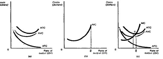
In the short run, some of the firm's inputs are fixed and others are variable. Building on this distinction, the short run theory of costs emphasizes two categories of costs—fixed and variable.

A fixed cost is the cost of a fixed input. In the short run, the fixed cost does not change as the firm's output level changes. Whether the firm produces more or less, it will pay the same for such things as fire insurance, local property taxes, and other costs independent of its output level. Fixed costs exist even at a zero rate of output. Perhaps the most important fixed cost is the opportunity cost of the firm's capital equipment and plant, that is, the next best alternative use of these resources. This cost exists even when the plant is idle. The only way to avoid fixed costs is to shut down and go out of business, an event that can occur only in the long run.

Variable costs are costs that change as the output level of a firm changes. When the firm reduces its level of production, it will use fewer raw materials and perhaps will lay off workers. Consequently, its variable costs of production will decline. Variable costs are expenditures on inputs that can be varied in short-run use. A third concept, total cost, is the sum of fixed and variable costs.

Fixed costs: Payments made to fixed inputs.

Variable costs: Payments made to variable inputs that necessarily change as output changes.

Total cost: All the costs of a firm's operations, including fixed and variable costs.

It is useful to determine the cost of producing each unit of output (each car, backpack, or ton of soybeans) in the short run as the level of output is increased or decreased.

The fixed cost per unit is called average fixed cost (AFC) and is found by dividing the total fixed cost by the firm's total output of the good (referred to as q). Since fixed costs are the same at all levels of output, AFC will decline continuously as output increases. This relation is shown graphically in Figure la.

Figure 1. Short-Run Cost Curves of the Firm

(a) The behavior of average fixed cost (AFC) average variable cost (AVC) and average total cost (ATC) as output changes ATC is the sum of AVC and AFC.

(b) The behavior of the firm s marginal costs (MC) as output increases MC ultimately raises as the short run capacity limit of the firm is approached at q.

(c) All the short-run cost curves. Notice in particular the U shape of the ATC curve ATC is high either where the firm’s plant is underutilized at low rates of output or overutilized at high rates of output.

 

Average variable cost (AVC) is found by dividing total variable cost by the firm's output. It is also drawn in Figure la, it ordinarily has a U shape.

Average total cost (ATC) — the actual short run cost to the firm of producing each unit of output — is total cost divided by total output.

Average total cost can also be found by adding average fixed costs and average variable costs. Thus, in Figure la, the ATC curve is shown as the sum of the AFC and AVC curves. Average total cost is sometimes referred to as unit cost.

Although the average total cost curve provides useful information, economic decisions are actually made at the margin. In considering a change in the level of production, firms must determine what the marginal cost of the change will be.

Marginal cost (MC) is the cost of producing each additional unit of output, it is found by dividing the change in total costs by the change in output. The result of such calculations is a marginal cost curve, shown in Figure 1b. Marginal cost first declines as output rises, reaches a minimum, but then rises because it becomes increasingly hard to produce additional output with a fixed plant. Extra workers needed to produce additional output begin to get in each other's way; inefficiencies proliferate as workers must take turns using machines; storage room for inputs and outputs becomes filled.At some point the firm's maximum output from its fixed plant will be reached (shown at q).

Figure lc brings all the short-run cost curves together. Notice that the ATC curve is U shaped. At low levels of output a firm does not utilize its fixed plant and equipment very effectively. The firm does not produce enough relative to the fixed costs for its plant, causing the average total cost to be high. At high levels of output the firm approaches its capacity limit (q). The inefficiencies of overloading the existing operation cause marginal costs to rise, raising the average total cost. These two effects combine to yield a U-shaped average total cost curve. Either low or high utilization of a fixed plant leads to high average total cost. The minimum point on the ATC curve, q, represents the lowest average total cost — the lowest cost per unit for producing the good. This represents the best short-run utilization rate for the firm.

Average fixed cost: Fixed cost divided by the level of output.

Average variable cost: Variable costs divided by the level of output.

Average total cost: Total costs divided by the level of output, or average fixed cost plus average variable cost, unit cost.

Marginal cost: The extra costs of producing one more unit of output the change in total costs divided by the change in output.

Table 1 provides a shorthand reference to all these concepts.

Table 1

Short-Run Cost Relations

Terms	Symbols	Definition
Average fixed cost=Fixed cost/Total output	AFC=FC/q	A fixed cost does not vary with output but the average fixed cost per unit declines as output rises
Average variable cost=Variable cost/Total output	AVC=VC/q	A variable cost changes as output changes
Average total cost=Total cost / Total output Average total cost=Average fixed cost + Average variable cost	ATC=TC/q ATC=AFC+AVC	Total cost is the sum of fixed and variable costs. Average total cost per unit forms a U-shaped curve when graphed from very low to very high output levels
Marginal cost=Change in total cost/Change in output	MC = ∆TC/∆q	Marginal cost rises as the short run capacity of afirm’s fixed plant is approached

Diminishing Returns

The behavior and shape of the short-run marginal cost and average total cost curves can he understood more completely with the law of diminishing marginal returns. The law of diminishing marginal returns states that as additional units of a variable input are combined with a fixed amount of other resources, die amount of additional output produced will start to decline beyond some point. The returns — additional output — that result from adding the variable input will ultimately diminish.

Law of diminishing marginal returns: A relation that suggests that as more and more of a variable input is added to a fixed input the resulting extra output decreases, eventually to zero.

Example:

A standard example comes from agriculture, we experiment by adding laborers to a fixed plot of land and observe what happens to output. To isolate the effect of adding additional workers (the variable input), we keep all inputs except labor fixed and assume that the technology does not change.

Table 2 is a numerical analysis of the results of such an experiment. The first column shows the amount of the variable input — labor — that is used in combination with the fixed input — land. The simplified numbers for total product and marginal product represent real measures of output such as torn of soybeans grown.

Marginal product is the change in total product caused by the addition of each additional worker. At first, as workers are added, total product expands rapidly. The first three workers show increasing marginal products (10, 12, and 14 extra tons of soybeans with the addition of each worker). Diminishing marginal returns set in, however, with the addition of the fourth worker. That is, the marginal product of the fourth worker is 13 tons, down from the 14-ton marginal product gained by adding the third worker. Marginal product continues to decline as additional workers are added to the plot of land. This squares with our earlier definition of the law of diminishing marginal returns. As additional units of a variable input are added to a fixed amount of other resources, beyond some point the amount of additional output produced will start to decline. In fact, the addition of the ninth and tenth workers leads to reductions in total product. Marginal product in these cases is negative, meaning that the addition of these workers actually reduces output. It becomes more and more difficult to obtain increases in output from the fixed plot of land by adding workers. At some point the workers simply get in each other's way.

Table 2

Law of Diminishing Marginal Returns

Variable Input (units of labor)	Total Product (tons) Marginal Product (tons)	Average Product (tons)
	0 0
	10 10	10.00
	22 12	11.00
	36 14	12.00
	49 13	12.25
	60 11	12.00
	70 10	11.67
	75 5	10.71
	78 3	9.75
	76 -2	8.44
	70 -6	7.00

If units of a variable input (labor) are added one at a time to production with a fixed plant (growing soybeans with no change in technology on a fixed plot of land), the total product, marginal product and average product all increase at first. But eventually as more workers are added they begin to get in each other’s way. Total output gained by adding more workers drops as predicted by the law of diminishing marginal returns.

 

The last column in the table introduces the concept of average product, which is total product divided by the number of units of the variable input. It is the average output per worker. Average product increases as long as marginal product is greater than average product. Thus, average product increases through the addition of die fourth worker. The marginal product of the fifth worker is 11, which is less than the average product for five workers, and beyond this point the average product falls.

Total product: The total amount of output that results from a specific amount of input

Marginal product: The extra output that results from employing one more unit of a variable input.

Average product: The output per unit of a variable input, total output divided by the amount of variable input.

Figure 2 graphically illustrates the law of diminishing marginal returns with the data from Table 2. Figure 2a illustrates the total product curve. Total product increases rapidly at first as the marginal product of the first three workers increases. Diminishing returns set in with the fourth worker, and thereafter the total product increases less rapidly. Beyond eight workers, the total product curve turns down and starts to decline. The maximum total product is reached with eight workers. The marginal product and average product curves are shown in Figure 2b. The marginal product curve is simply the slope of the total product curve. It rises to a maximum at three workers and then declines as diminishing returns set in. Eventually, it becomes negative at eight workers, indicating that total product is decreasing. The average product curve rises when marginal product is greater than average product, and it declines when marginal product is less than average product.

Figure 2. Total, Average, and Marginal Product Curves

(a) Total product curve, plotting data from Table 2

(b) Average product and marginal product curves

Marginal product is the rate of change of the total product curve. The area of diminishing marginal returns begins when marginal product starts to decline. Average product rises when marginal product is greater than average product and it falls when marginal product is less than average product.

How can the law of diminishing marginal returns are applied to economic decision making. Consider the thinking of the farmer who owns the plot of land in this experiment. How many workers will he or she choose to hire. Before the area of diminishing marginal returns is reached, additional workers have an increasing marginal product. The farmer will add these workers and will go no further in hiring than the point where the marginal product falls to zero. Even if labor were free, the farmer would not go beyond this point because there would be so many workers on the land that the marginal product of an additional worker would be negative and the total product would decline. This implies that it is rational for the farmer to operate somewhere in the area of diminishing marginal returns.

Precisely how many workers will maximize profits. The answer depends on the cost of the workers. Assume that each worker is paid a wage rate equivalent to 4 units of output. The farmer will compare the marginal product of each worker with the wage rate. The fourth worker adds 13 units of output and costs the farmer the equivalent of only 4 units. In fact, the marginal product of the first seven workers exceeds their wage rate. However, the marginal product of the eighth worker is 3 units of output, which is less than the wage rate. The rational farmer will therefore hire seven workers. This is the law of diminishing marginal returns in action. It points the farmer toward the rational utilization of factors of production.