Diminishing Marginal Returns and Short-Run Costs

MC = Increase in total cost / Increase in output

Increase in total cost = Increase in the number of units of the variable input x Price of the variable input

 

MC=Increase in quantity of variable input x Price of variable input / Increase in output

We know that marginal product is defined as:

MP= Increase in output / Increase in the quantity of the variable input

Thus the first term in the MC expression is the reciprocal of marginal product. MC can further be rewritten as:

MC= Price of variable input / Marginal product of variable input

 

This means that marginal cost is inversely related to marginal product. That is, if the price of the variable input is constant, then increases in marginal cost are associated with decreases in marginal product. The law of diminishing marginal returns is equivalent to increasing marginal cost.

Example:

Table 3 presents a numerical illustration of how the law of diminishing marginal returns affects a firm's short-run costs. Columns (2), (3), and (4) show how total costs behave as output increases in the short run, and columns (5), (6), and (7) show the behavior of the corresponding average cost concepts.

In this example, we keep the numbers low for simplicity. Total fixed cost is, constant at $10 per day, average fixed cost per unit is the total fixed cost divided by output. Fixed costs must be paid in the short run regardless of whether the firm operates. The level of average fixed cost falls continuously as output is increased.

Table 3

Short-Run Cost Data for a Firm

Total Cost Data (per day)	Average and Marginal Cost Data (per day)
(1) Output (units)	(2) Total Fixed Cost	(3) Total Variable Cost	(4) Total Cost (2)+(3)	(5) Average Fixed Cost (2)/(1)	(6) Average Variable Cost (3)/(1)	(7) (8) Average Total Marginal Cost Cost (4)/(1) ∆(4)/∆(1)
	$10.00	$0	$10.00	$0	$0	$0 $1.60
	10.00	1.60	11.60	10.00	1.60	11.60 1.40
	10.00	3.00	13.00	5.00	1.50	6.50 1.35
	10.00	4.35	14.35	3.34	1.45	4.78 1.30
	10.00	5.70	15.70	2.50	1.43	3.93 1.20
	10.00	6.90	16.90	2.00	1.38	3.33 1.10
	10.00	8.00	18.00	1.67	1.33	3.00 1.00
	10.00	9.00	19.00	1.43	1.29	2.71 0.90
	10.00	9.90	19.90	1.25	1.24	2.49 0.30
	10.00	10.20	20.20	1.11	1.13	2.24 0.65
	10.00	11.85	21.85	1.00	1.19	2.19 1.30
	10.00	13.15	23.15	0.91	1.20	2.11 1.50
	10.00	14.65	24.65	0.83	1.22	2.05 1.75
	10.00	16.40	26.40	0.77	1.26	2.03 2.05
	10.00	18.45	28.45	0.71	1.32	2.03 2.45
	10.00	20.90	30.90	0.67	1.39	2.06 2.90
	10.00	23.80	33.80	0.62	1.49	2.11 3.40
	10.00	27.20	37.20	0.59	1.60	2.19 3.95
	10.00	31.15	41.15	0.56	1.73	2.29 4.55
	10.00	35.70	45.70	0.53	1.88	2.41 5.25
	10.00	40.95	50.95	0.50	2.05	2.55

*∆= change in

The various concepts of short-run costs are expressed in both total and average terms. Columns (1) through (4) present the firm's total cost data; columns (5) through (8) present the cost data in average terms. Notice especially that short-run marginal cost ultimately rises because of the law of diminishing marginal returns.

 

Total variable cost is the sum of the firm's expenditures on variable inputs. Average variable cost is the total variable cost divided by output. Notice that total variable cost first increases at a decreasing rate and that after nine units of output it increases at an increasing rate.

Total cost is the sum of total fixed and total variable costs. Average total cost is the sum of average variable and average fixed costs, or simply total cost divided by output.

Marginal cost, shown in column (8), is the change in total cost that results from producing one additional unit of output. The behavior of marginal cost reflects the law of diminishing marginal returns. In this example, marginal cost falls through the production of the ninth unit of output and rises thereafter. The rising portion of the marginal cost schedule reflects diminishing marginal returns for additions of the variable input.

The data in Table 3 are plotted in Figure 3, which graphically demonstrates the behavior of short run cost curves. Figure 3a illustrates the concepts of total cost, and Figure 3b presents the corresponding average and marginal cost concepts. Notice in part b that MC intersects AVC and ATC at their minimum points. This is because marginal cost bears a definite relation to average variable cost and average total cost. In the case of average total cost, marginal cost lies below average total cost when average total cost is falling and above average total cost when average total cost is rising. Marginal cost is equal to average total cost at the point where average total cost is at a minimum. In Table 3, this occurs between the thirteenth and fourteenth units of output. At lower levels of output, the MC values in column (8) are less than the ATC values in column (7). ATC therefore declines. At higher levels of output, the MC values are greater than the ATC values, and ATC rises. The same analysis holds for the relationship between MC and AVC.

This same relation holds for average total cost and marginal cost, which both Table 3 and Figure 3 verify.

Figure 3. Short-Run Cost Curves

(a) Total cost data plotted from Table 3

(b) Average cost and marginal cost data

Notice the U-shaped average total cost curve. At low levels of output ATC is high because AFC is high and the firm does not utilize its fixed plant efficiently. At high levels of output ATC is high because MC is high as the firm approaches the capacity limit of its plant. These effects give ATC a U shape.

In sum, the firm's short-run cost curves show the influence of the law of diminishing marginal returns.

First, the firm has certain fixed costs independent of level of output. These costs correspond to what the firm must pay for fixed inputs, and they must be paid whether or not the firm operates.

Second, assuming the price of variable inputs is constant, marginal costs reflect the behavior of the marginal product of the variable input. As output rises, marginal costs first decline because marginal product is increasing and it requires less and less of the variable input to produce additional units of output. At some point, however, diminishing marginal returns set in, and it takes more and more of the variable input to produce additional units of output. When this happens, marginal costs start to rise.

Third, marginal cost will eventually rise above average variable cost and average total cost, causing these costs to raise as well, which results is a U-shaped average total cost curve.

 

Long-Run Costs

 

In the short run, some inputs are fixed and cannot be varied. These fixed inputs generally are characterized as a physical plant that cannot be altered in size in the short run. Short-run costs therefore show the relation of costs to output for a given plant. In the long run, however, all inputs are variable, including plant size. As economic time lengthens and the contracts that define fixed inputs can be renegotiated, a firm owner can adjust all parts of his or her operation. In fact, the scale of a firm's operations can be adjusted to best fit the economic circumstances that prevail in the long run, an owner can choose to arrange the organization in the best possible way to do business. Stated in terms of plant size, the owner will seek the plant size that minimizes long run costs of producing theprofit maximizing output.

Adjusting Plant Size

The choice of plant size affects production costs.

Example:

An owner might have the choice of four plants, such as those depicted in Figure 4. The ATC curves are short run average total cost curves that correspond to four different-sized plants. Which plant is best from the owner's point of view? The answer depends on the profit maximizing level of output. If the firm wants to produce less than q₁, the plant represented by ATC₁ is the lowest cost plant for those levels of output. For outputs between q₁ and q₂, ATC₂ is the lowest-cost plant. For outputs between q₂ and q₃, ATC₃ is the lowest-cost plant. For even larger outputs — beyond q₃ — the plant represented by ATC₄ is the lowest-cost plant.

In effect, the owner's best course of action is depicted by PLAN in Figure 4. Given that inputs can be varied to build any of these plants, the owner will move along a path such as PLAN gradually expanding output by expanding plant size, seeking the lowest cost way to produce the profit-maximizing output in the long run.

Figure 4. Adjusting Plant Size to Minimize Cost

The figure shows short-run average total cost curves for four plant sizes. If these are the only alternative plant sizes available, the long-run average total cost (or planning) curve will be given by PLAN. That is, starting with plant size P, the rational owner expands plant size to L, A, and then N in the long run. Each point represents movement to a larger and lower-cost plant size.

 

To determine the optimum long run plant size, we introduce a new concept long-run average total cost (LRATC). This measure shows the lowest-cost plant for producing each level of output when the firm can choose among all possible plant sizes.

Long-run average total cost: The lowest possible cost per unit of producing any level of output when all inputs can be varied.

In Figure 4, PLAN is the long-run average total cost curve when only four plants are possible. In the long run, however, more than four plant sizes are possible. Indeed, the number of possible plant sizes is unlimited. In effect, the owner sees the world of possibilities in terms of a long-run average total cost (or planning) curve such as that drawn in Figure 5.

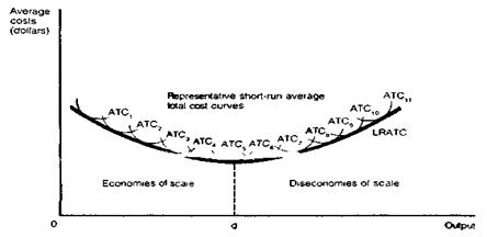
Figure 5. Long-Run Average Total Cost Curve

LRATC is planning curve of the firm owner. It shows how plant size can be adjusted in the long run when all inputs are variable. The plant size shown at q represents the lowest possible unit cost of production in the long run. Economies of scale prevail before q on the curve and diseconomies of scale prevail past q.

The long-run average total cost curve is smoothly continuous and allows us to see the full sweep of a firm owner's imagination. On its downward course, the long-run average total cost curve is tangent to each short-run average total cost curve before the point of minimum cost for each given plant size. On its upward course it touches each short-run average total cost curve past the point of minimum cost. Only at the bottom of the long-run U - shape do the minimum points of the long-run and short-run average total cost curves coincide. In effect, the long-run average total cost curve is an envelope of short-run average total cost curves.