Заглавная страница Избранные статьи Случайная статья Познавательные статьи Новые добавления Обратная связь FAQ Написать работу КАТЕГОРИИ: ТОП 10 на сайте Приготовление дезинфицирующих растворов различной концентрацииТехника нижней прямой подачи мяча. Франко-прусская война (причины и последствия) Организация работы процедурного кабинета Смысловое и механическое запоминание, их место и роль в усвоении знаний Коммуникативные барьеры и пути их преодоления Обработка изделий медицинского назначения многократного применения Образцы текста публицистического стиля Четыре типа изменения баланса Задачи с ответами для Всероссийской олимпиады по праву 
Мы поможем в написании ваших работ! ЗНАЕТЕ ЛИ ВЫ?
Влияние общества на человека
Приготовление дезинфицирующих растворов различной концентрации Практические работы по географии для 6 класса Организация работы процедурного кабинета Изменения в неживой природе осенью Уборка процедурного кабинета Сольфеджио. Все правила по сольфеджио Балочные системы. Определение реакций опор и моментов защемления |
Boundary problem for system of the second order. Green function.Содержание книги
Поиск на нашем сайте
We consider a system of the second order boundary value problem of the type
with the boundary conditions u (a) = and the continuity conditions of u and u’ at c and d. Here, f and g are continuous functions on [ a; b ] and [ c; d ], respectively. The parameters r; are real finite constants. Such type of systems arises in connection with the Green function. L[y] = 0, U1[y] = 0, U2[y] = 0. has only trivial solution. Let (λ1, λ2) 6= (0, 0) be such that a1λ1 + a2λ2 = 0 and let φ1 be solution of L[y] = 0 satisfying φ1(a) = λ1 and φ′1(a) = λ2. Choose another solution φ2 of L[y] = 0 similarly. This way of choosing φ1 and φ2 make sure that both are non-trivial solutions. Note that φ1 and φ2 form a fundamental pair of solutions of L[y] = 0, since we assumed that homogeneous BVP has only trivial solutions. By Lagrange’s identity (5.20), we get d/dx[p(φ′1φ2 − φ1φ′2)= 0. This implies p(φ′1φ2 − φ1φ′2) ≡ c, a constant and non-zero, (5.44) as a consequence of (φ′1φ2 − φ1φ′2) being the wronskian corresponding to a fundamental pair of solutions. Green’s function is then given by G(x, ξ):=1/c
21) Reduction of equation to canonical form. Canonical form in a differential form that is defined in a natural (canonical) way; Finding a canonical form is called canonization. Canonical differential forms include the c anonical one-form and canonical symplectic form For instance, the expression f(x) dx from one-variable calculus is called a 1-form, and can be integrated over an interval [ a, b ] in the domain of f Likewise, a 3-form f(x, y, z) dxdydz represents something that can be integrated over a region of space Canonical one-form is a special 1-form defined on the cotangent bundle T * Q of a manifold Q. The exterior derivative of this form defines a symplectic form giving T * Q the structure of a symplectic manifold. The tautological one-form plays an important role in relating the formalism of Hamiltonian mechanics and Lagrangian mechanics. The tautological one-form is sometimes also called the Liouville one-form, the Poincaré one-form, the canonical one-form, or the symplectic potential. A similar object is the canonical vector field on the tangent bundle. In canonical coordinates, the tautological one-form is given by Equivalently, any coordinates on phase space which preserve this structure for the canonical one-form, up to a total differential (exact form), may be called canonical coordinates; transformations between different canonical coordinate systems are known as canonical transformations. The canonical symplectic form is given by The extension of this concept to extended to general fibre bundles is known as the solder form.
22) Autonomic system properties. Trajectory, phase space. A system of ordinary differential equations which does not explicitly contain the independent variable (time). The general form of a first-order autonomous system in normal form is:
or, in vector notation, A non-autonomous system A complex autonomous system of the form (1) is equivalent to a real autonomous system with 2n unknown functions
The essential contents of the theory of complex autonomous systems — unlike in the real case — is found in the case of an analytic f(x) Consider an analytic system with real coefficients and its real solutions. Let x Local properties of solutions. 1) If Φ(t) 2) Existence: For any
3) Smoothness: If f⋲ 4) Dependence on parameters: Let, f=f(x,α),α⋲ 5) Let
A substitution of variables x = Φ(y) in the autonomous system (1) yields the system (2)
where is the Jacobi matrix.
23) Solution properties of autonomic systems.
|
||||
|
|
Последнее изменение этой страницы: 2016-08-14; просмотров: 178; Нарушение авторского права страницы; Мы поможем в написании вашей работы! infopedia.su Все материалы представленные на сайте исключительно с целью ознакомления читателями и не преследуют коммерческих целей или нарушение авторских прав. Обратная связь - 18.225.54.147 (0.008 с.) |


 and u (b) =
  (2)
(2)
 and similarly the expression: f (x, y, z) dx ∧ dy + g (x, y, z) dx ∧ dz + h (x, y, z) dy ∧ dz is a 2-form that has a surface integral over an oriented surface S:
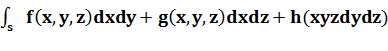
 idqi
idqi idpi
idpi =
=  (
( ) j=1,…,n
 =f(x). (1)
 =t. Historically, autonomous systems first appeared in descriptions of physical processes with a finite number of degrees of freedom. They are also called dynamical or conservative systems
 (Re x)= Re f(x),
  Φ (t) be an (arbitrary) solution of the analytic system (1), let ∆ =(
 ) be the interval in which it is defined, and let x(t;
  ,
,  ) be the solution with initial data x
  =
=  and f
and f 
 (G). The point
  G is said to be an equilibrium point, or a point of rest, of the autonomous system (1) if f(
 0. The solution, Φ(t)
 corresponds to such an equilibrium point
 is a solution, then Φ(t+c) is a solution for any c
  .
. ,
,  G,a solution x(t;
  .
. , then Φ(t)⋲
  .
. C R,where
  (G*
(G*  ),p≥1, x(t;
  )⋲
)⋲  = const in W.
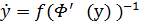 f(Φ(y)), where
  (y) is the Jacobi matrix.