Заглавная страница Избранные статьи Случайная статья Познавательные статьи Новые добавления Обратная связь FAQ Написать работу КАТЕГОРИИ: ТОП 10 на сайте Приготовление дезинфицирующих растворов различной концентрацииТехника нижней прямой подачи мяча. Франко-прусская война (причины и последствия) Организация работы процедурного кабинета Смысловое и механическое запоминание, их место и роль в усвоении знаний Коммуникативные барьеры и пути их преодоления Обработка изделий медицинского назначения многократного применения Образцы текста публицистического стиля Четыре типа изменения баланса Задачи с ответами для Всероссийской олимпиады по праву 
Мы поможем в написании ваших работ! ЗНАЕТЕ ЛИ ВЫ?
Влияние общества на человека
Приготовление дезинфицирующих растворов различной концентрации Практические работы по географии для 6 класса Организация работы процедурного кабинета Изменения в неживой природе осенью Уборка процедурного кабинета Сольфеджио. Все правила по сольфеджио Балочные системы. Определение реакций опор и моментов защемления |
Fundamental system of solutions.Содержание книги
Поиск на нашем сайте
Definition. System of n linearly independent solutions of system Theorem. The system (1) has a fundamental system of solutions. If
Concept of the fundamental matrix. Ostrogradsky-Liouville formula. We consider the system y 1(t) ,y 2 (t),.. ,yn (t) (2) Y(t) = and the Wronskian. If (2) is linearly independent, then detY(t) =W(t) Y (t) is called an integral or a fundamental matrix for the system (1). If Y (t 0) = E, the matrix is called integral normalized at the point t = t 0. Theorem. If Y (t) is integral matrix of vector equation (1), we have detY(t)=detY(t0)*exp the Ostrogradsky-Liouville formula. Linear transformations
Theorem. The general solution of the inhomogeneous vector equation Yh=Yp+Yinh (5)
17) Fundamental matrix. Liouville formula A square matrix Φ(t) whose columns are formed by linearly independent solutions x 1(t), x 2(t),..., xn (t) is called the fundamental matrix of the system of equations. It has the following form:
where xij (t) are the coordinates of the linearly independent vector solutions x 1(t), x 2(t),..., xn (t). Φ(t) is nonsingular, i.e. there always exists the inverse matrix Φ −1(t). Since the fundamental matrix has n linearly independent solutions, after its substitution into the homogeneous system we obtain the identity Ф’(t) Ф’(t) The general solution of the homogeneous system is expressed in terms of the fundamental matrix in the form
Ф(t)
on an interval I of the real line, where A (x) for x ∈ I denotes a square matrix of dimension n with real or complex entries. Let Φ denote a matrix-valued solution on I, meaning that each Φ(x) is a square matrix of dimension n with real or complex entries and the derivative satisfies Ф’(t) Let trA(ξ)= A(ξ) = (ai, j (ξ))i, j ∈ {1,...,n}, the sum of its diagonal entries. If the trace of A is a continuous function, then the determinant of Φ satisfies detФ(x) for all x and x 0 in I.
Integration of linear inhomogeneous system with quasi-polynomial right side.
Theorem: Condition: The vector-function
Statement: vector- function
Proof: adding the equality
We get that Def:Vector-function
Statement: If Proof: right size of (1) we can submit Particular sol. of system
Solution of sourse function is
19) Studying of different cases (resonance and in resonance cases) Theorem 1 (Non-resonance). Assume that 'ϕ(λ) has no roots on the imaginaryaxis, g 2 BC and p 2 C. Then equation has at least one bounded solution if and only if p? C0 + BC: To state the result in the case of resonance we follow and define the notion of upper and lower average. Given p?C0 + BC,
It is easy to verify that −1 < AL (p) <= AU (p) < +1: Moreover, if p is periodic the identity AL (p) = AU (p) = p holds and the concept of average is recovered. Theorem 2 (Resonance). Assume that λ = 0 is a simple root of ϕ(λ) and there are no other roots on the imaginary axis. In addition, g? BC and p? C. Then a sufficient condition for the existence of a bounded solution p? C 0 + BC; As mentioned in the introduction, this theorem extends results.
and it was proved that if g? BC there exists a bounded solution if and only if p= p*+p** with p *? C 0 g (−∞) < inf p** <= sup p **<g(+∞)
|
||||
|
|
Последнее изменение этой страницы: 2016-08-14; просмотров: 476; Нарушение авторского права страницы; Мы поможем в написании вашей работы! infopedia.su Все материалы представленные на сайте исключительно с целью ознакомления читателями и не преследуют коммерческих целей или нарушение авторских прав. Обратная связь - 216.73.216.2 (0.009 с.) |

 1(t),
1(t),  2(t),…
  = A(t)
  (1) is a fundamental system of solutions or basis.
 i
i 
 (2)
(2) = B(t)
  (3)
(3) = A(t)
  +
+  (t) (4)is equal to the total solution (5)of the homogeneous equation (1) and a particular solution of the inhomogeneous vector equation (4)
 A(t)Ф(t)
 A(t)Ф(t)

 Ф’(t)
Ф’(t)  (t)= Ф(t)C where C is an n -dimensional vector consisting of arbitrary numbers. The fundamental matrix Φ(t) for such a system of equations is given by
 Liouville formula. Consider the n -dimensional first-order homogeneous linear differential equation
 A(t)Ф(t) x ∈ I
 ξ ∈ I
ξ ∈ I
 (x)=A
(x)=A  (x)+
(x)+  (x), (L[
  (x) has the form
  (x)
(x)  +…+
+…+  (x) and vector-function
  (x)
(x)  (x) is the solution of followin inhomogeneous systems
 (x)
(x)  (x)
(x) 
 (x)
(x)  +
+  (x)
(x)  …+
…+  (x)
(x)  +
+  (x)
(x) (x)*
(x)*  , where
  (x)- quasi-polinom
 (x)=
(x)=  (x)*
(x)*  +
+  (x)*
(x)*  (1) then there
  (x) and
  (x) polinoms of r=k degree such that Vector-function
  (x)*
(x)*  +
+  (x)*
(x)*  is particular solution of inhomogeneous linear system.
 (x)*
(x)*  +
+  (x)*
(x)* 
 (x)=
(x)=  (x)=
(x)=  (x) *
(x) *  (x),
(x),  (x) quasi-polinoms
 (x)
(x)  (x)*
(x)*  (x)*
(x)*  (p):=
(p):= 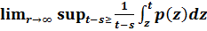
 (p):=
(p):= 
 (−∞) <
  (p) <=
  (p) < g (+∞):
 + c
+ c