Заглавная страница Избранные статьи Случайная статья Познавательные статьи Новые добавления Обратная связь FAQ Написать работу КАТЕГОРИИ: ТОП 10 на сайте Приготовление дезинфицирующих растворов различной концентрацииТехника нижней прямой подачи мяча. Франко-прусская война (причины и последствия) Организация работы процедурного кабинета Смысловое и механическое запоминание, их место и роль в усвоении знаний Коммуникативные барьеры и пути их преодоления Обработка изделий медицинского назначения многократного применения Образцы текста публицистического стиля Четыре типа изменения баланса Задачи с ответами для Всероссийской олимпиады по праву 
Мы поможем в написании ваших работ! ЗНАЕТЕ ЛИ ВЫ?
Влияние общества на человека
Приготовление дезинфицирующих растворов различной концентрации Практические работы по географии для 6 класса Организация работы процедурного кабинета Изменения в неживой природе осенью Уборка процедурного кабинета Сольфеджио. Все правила по сольфеджио Балочные системы. Определение реакций опор и моментов защемления |
General properties of solutions. Continuity, differentiation of solutions of parameter axis and initial data.Содержание книги
Поиск на нашем сайте
Consider the IVP with a parameter s ∈ Rm
where f: Ω → Rn and Ω is an open subset of (t, x, s) = (t, x1,.., xn, s1,..., sm). For any s ∈ Ωs ={(t, x) ∈ S = {s ∈ = {s ∈ Then the IVP can be considered in the domain Ωs for any s ∈ S. We always assume that the set S is non-empty. Assume also in the sequel that f (t, x, s) is a continuous function in (t, x, s) ∈ Ω and is locally Lipschitz in x for any s ∈ S. For any s ∈ S, denote by x (t, s) the maximal solution of (1) and let Is be its domain (that is, Is is an open interval on the axis t). Hence, x (t, s) as a function of (t, s) is defined in the set U ={(t, s) ∈ Theorem 1. Under the above assumptions, the set U is an open subset of the function x (t, s): U → Differentiability Of solutions. A property of solutions of differential equations, that the solutions posses a specific number of continuous derivatives with respect to the independent variable and the parameter appearing in the equation. Consider an equation of the type (x may also be a vector):
where μ is a parameter (usually also a vector), and let x(t, μ) be a solution of (1) defined by the initial condition
Linear equations of the n-th order. Basic properties. Let’s consider the differential equation
which coefficients p 1(x),..., pn (x) and the constant term f (x) are continuous on the interval J ⊆ (− ∞,∞). It is required to find a solution of equation (1) with conditions y(x0)=y0, y’(x0)= The problem (1), (2) is called Cauchy problem. Theorem 1. Let the coefficients pi (x), i = 1, n of equation (1) and the right side f (x) be continuous on the interval J.Then it has a unique solution y = ϕ(x)∈ and we call L as n order linear differential operator (acting in Concept of operator generalizes the notion of function. In this situation, the operator L for each function y ∈ is called a linearity of operator.If in equation (1) f (x) vanishes, we obtain the equation L (y) = 0, (5) which is called homogeneous. And the equation (1) is called a linear inhomogeneous. Further, we consider the homogeneous equation (5). Theorem 2. Linear combination solutions of equation (5) is a solution. 10) Linear homogeneous equations, Solution properties. the Euler method which is a method of constructing a fundamental system of solutions for the equation is
Following Euler we find solutions of equation (1) in the form y =
Equation (2) is called characteristic for the differential equation (1). It is considered separately the different cases. 1) The roots of the characteristic polynomial l( λ ) are real and different. 2) The roots of the characteristic polynomial are different, but among of them there are complex roots. 3) The roots of the characteristic equation are real, but among of them there are multiple. To multiple root λ =λ * multiplicity " k " corresponding to " k " linearly independent solutions of the form y 1= 4) In the general case can also be multiple complex roots. Note that if the multiplicity of the root α + i β is e, that multiplicity of the adjoint root as well e. Therefore, such pair of roots corresponding to the following linearly independent solutions e α x cosβx, xe α x cosβx, …….., x l -1 e α x cosβx e α x sinβx, xe α x sinβx, …….., x l -1 e α x sinβx
|
||||||||
|
|
Последнее изменение этой страницы: 2016-08-14; просмотров: 268; Нарушение авторского права страницы; Мы поможем в написании вашей работы! infopedia.su Все материалы представленные на сайте исключительно с целью ознакомления читателями и не преследуют коммерческих целей или нарушение авторских прав. Обратная связь - 18.224.169.152 (0.008 с.) |

 (1)
(1) . Here the triple (t, x, s) is identified as a point in
  , consider the open set
 : (t, x, s) ∈ Ω} Denote by S the set of those s, for which Ωs contains (t0, x0), that is,
 : s ∈ S, t ∈ Is}
 is continuous.
 = f(t, x, μ)(1)
 =f(x ) (1)
 , ….
, ….  (2)
(2) (J) satisfying to the initial conditions (2). We introduce a special notation for the left side of equation (1) L (y) ≡
  + p (x)
  pn (x) y (3)
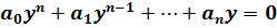 (1)
(1) , where λ is a constant. We prove that equation (1) has a solution of the form y =
 , y 2=x
  =
=