Заглавная страница Избранные статьи Случайная статья Познавательные статьи Новые добавления Обратная связь FAQ Написать работу КАТЕГОРИИ: ТОП 10 на сайте Приготовление дезинфицирующих растворов различной концентрацииТехника нижней прямой подачи мяча. Франко-прусская война (причины и последствия) Организация работы процедурного кабинета Смысловое и механическое запоминание, их место и роль в усвоении знаний Коммуникативные барьеры и пути их преодоления Обработка изделий медицинского назначения многократного применения Образцы текста публицистического стиля Четыре типа изменения баланса Задачи с ответами для Всероссийской олимпиады по праву 
Мы поможем в написании ваших работ! ЗНАЕТЕ ЛИ ВЫ?
Влияние общества на человека
Приготовление дезинфицирующих растворов различной концентрации Практические работы по географии для 6 класса Организация работы процедурного кабинета Изменения в неживой природе осенью Уборка процедурного кабинета Сольфеджио. Все правила по сольфеджио Балочные системы. Определение реакций опор и моментов защемления |
Lecture purpose: studying of methods of creation of statistical models of the CTS elements.Содержание книги
Поиск на нашем сайте Plan of a lecture: 1. Method of the smallest squares. 2. Active (factorial) and passive experiment. 3. Fractional factorial test 4. Orthogonal central composite plan. 5. Equation of regression of an object 6. Matrixes of planning of a two-factor experiment. 7. Check of adequacy of model. 8. Assessment of the importance of factors,
In case of development of statistical models of CTS modules the task of the detailed description of regularities of the processes happening in an object since its mathematical description is under construction in the form of regression dependences of output parameters of an object on entrance isn't set and represents the linear or nonlinear polynomial equations. Coefficients of the polynomial equations find by handling of the experimental data obtained on production or on the specified physical and chemical model of an object with use of a method of the smallest squares. Thus, approach to a technological object as to "a black box", i.e. without the processes which are taking place in the object allows to create model with the minimum costs for data collection and processing. The essence of a method of the smallest squares is that through a number of experimental points carry out such dependence (Y=f (X1,X2, Xm)), which amount of squares of deviations from experimental values in case of the corresponding X1, X2 and Xm values – is minimum (see Fig. 4.14).
Fig. 4.14. Illustration of a method of the smallest squares
The type of dependence of Y=f (X1,X2, Xm) can be various. However usually dependence of Y=f (X1,X2, Xm) represents a polynomial: Xm – is minimum (see Fig. 4.14).
where ai – polynomial coefficients; Xi – changeable factors; m – quantity of factors. Coefficients of a polynomial of ai at which the sum of squares of differences of experimental (YIE) and settlement (YIR) values will be minimum (the equation 4.25) can be calculated with use of various mathematical methods (the solution of system of the linear equations, minimization, etc.).
It should be noted that the method of the smallest squares is rather widely used when processing experimental data since allows not only to determine parameters of the polynomial dependences which are describing work of an object, and not making physical sense but also to specify parameters of physical and chemical models. For example, when calculating coefficient of a heat transfer (the equation 4.21) the coefficients of a thermalizes (aX and aG) depending on parameters of the movement of a stream of hot and cold heat carriers which can be calculated on criteria dependences which are kinds of physical and chemical models are used:
where the A, B, C and D parameters are in result of processing of experimental data by method of the smallest squares. It is possible to give the equation of dependence of a constant of speed of chemical reaction of the steam conversion of monoxide of carbon for the iron chromic of catalysts in the range of temperatures 400-500OC which is the cornerstone of physical and chemical model of the reactor as other example:
where values of coefficients: "34000", "4,57" and "10,2" have also been found by data processing of an experiment on studying of kinetics of steam conversion of monoxide of carbon method of the smallest squares. The polynomial equation of dependence of an isobaric thermal capacity on temperature (the equation 4.13) which is used in physical and chemical model can be one more example. Coefficients of this equation have been also received by processing of experimental data by method of the smallest squares. Except specified, it is possible to give still a set of similar examples where concepts the statistical model and physical and chemical model have rather closely intertwined among themselves. However, it should be noted that the side between physical and chemical and statistical models is very thin since in fact, distinctions depend only on depth of consideration of the processes happening in a real object and completeness of their mathematical description. Feature of physical and chemical models is that at their use process is considered at two levels: lower – the level of change of parameters of processes and properties of streams, and, top – the level describing features of processes. For example, Arrhenius's equation is rather widely used as dependence of a constant of speed of various chemical reactions on temperature:
where the coefficients of k0 and EAKT (making physical sense) can be determined, for example, for process of steam conversion of methane, processing of experimental data by method of the smallest squares. For other process coefficients and EAKT will have other values, but the type of the equation will remain the same. Moreover, experimentally it is also theoretically proved that, for example, at decrease of the activity of the catalyst the size of energy of activation (EAKT) will remain invariable, and only the k0 parameter will change. Thus, knowing a general view of physical and chemical dependence and value of two constants, the possibility of the description of rather difficult dependence of a constant of speed on temperature in a wide interval of change of parameters of process appears. In case of use of statistical models an object is considered as a unit without specification of the processes happening in him, i.e. in the form of "a black box" for which functions of transformation of input parameters during the week-end. are defined. These functions of transformation can have various appearance even for identical technological objects since don't make any physical sense. Moreover, if installation for which the statistical model has been made passes into an operating mode which parameters weren't used by drawing up model, then her statistical model has to be constructed anew since application of statistical model is limited to limits of a variation of input and output parameters within the data used by drawing up model (see Fig. 4.15), i.e. in limits for which her adequacy to a real object has been proved.
Fig. 4.15. Illustration of limits of applicability of statistical model
In Fig. 4.5. it is visible that dependence of output parameter (Y) on entrance (Xm) well describes experimental points only within a variation of input parameter from Xmin to Xmax, and output parameter from Ymin to Ymax. Outside a variation of parameters dependence can pass randomly. Thus, unlike physical and chemical model, the statistical model can't be extrapolated out of limits of a variation of parameters. For expansion of parameters of a variation it is necessary to collect additional data and to anew constitute model. Usually carry the models received by data processing of an active (factorial) or passive experiment on a real object or by means of adequate model to statistical models. In case of active factorial test if linear dependences between output and entrance variables are observed, then plans of the first order are used: complete factorial test (CFT) and fractional factorial test (FFT). If dependences between output and entrance variables of active factorial test have obviously nonlinear nature, for receipt of the mathematical description of an object use composite plans of the second order, for example, the orthogonal central composite plan (OCCP). In case of data processing of a passive experiment receive the regression equation which complexity is determined depending on complexity of an object, quantity of basic data and required accuracy. PFE in comparison with passive statistical methods of receipt of the mathematical description of model has an advantage in what allows to obtain a maximum of information on an object in case of the minimum quantity of experiences. However, PFE is generally applied to receipt of statistical model of an object on the basis of its physical and chemical model or if on installation there is an opportunity to plan change of the technological modes without prejudice to production. One more condition of use of PFE is importance and mutual independence of initial parameters. In a general view, the equation of regression of an object can be provided by means of a polynomial:
where ai – polynomial coefficients; Xi – changeable factors; m – quantity of factors. In PFE all factors vary at two levels: upper (it is designated: +1) and lower (it is designated:-1). When carrying out experiments various combinations of factors at the chosen levels are implemented. For accounting of mutual influence of two factors use their pair works. In this case, the quantity of series of experiences can be counted on a formula: N=2m [4.30] The example of a matrix of planning of a two-factor experiment is provided in Table 4.2. Table 4.2 Matrix of planning of a two-factor experiment
When handling results of PFE coefficients of the regression equation, adequacy dispersion, dispersion of an average, criterion of Fischer by whom adequacy of the regression equation, etc. is determined are determined. Upon termination of data processing the conclusion about adequacy of model is drawn. If the model is inadequate, for example, change basic data, change a type of the regression equation, and carry out handling anew. However, methods of data processing of an active experiment aren't always applicable for creation of models of CTS modules based on production data since in the conditions of the real industrial plant it is rather difficult to observe the required intervals of a variation of parameters set in the plan. For this reason, the greatest distribution for creation of statistical models of CTS modules was gained by methods of handling of production data by method of a passive experiment. For receipt of statistical model on the basis of data processing of a passive experiment, data collection is made from the operating installation and present them in the form provided on Table 4.3. Table 4.3. Form of representation of basic data
It was specified above that the statistical model "works" only within a variation of parameters therefore collection of basic data needs to be made for all the set operating modes of installation in the widest limits of their variation. Usually, the plan of change of parameters is developed by means of the methods accepted in PFE since these methods allow to obtain the maximum information on an object with the minimum quantity of changes of parameters. In case of data collection it is necessary to consider the principle: the more it is collected data – the better. Special attention should be paid on an installation operating mode since it is possible to constitute statistical model of an element of technological installation only for the stationary modes of its work. However, really, after change of any parameters, the stationary operating mode of installation is reached only through certain time. Moreover, if installation has no ACS, then process of achievement of a stationary operating mode by it can be slowed down due to transition processes. For this reason, before data collection it is necessary to reduce as much as possible influence of a management system of the surveyed installation element on change of the modes of its work, for example, as transfer of an element of installation to manual control. If transfer to manual control is impossible, then in this case it is necessary to determine time of stabilization of an operating mode of installation upon termination of change of parameters of the technological mode and to begin data collection only after this time. Because the main operating mode of any technological installation is the dynamic mode, i.e. installation constantly is in process of transition of one condition in another (the question only consists in the speed of this transition), in case of collection of the current technological parameters it is necessary to determine by sizes of an expense, temperature, structure, etc. approximate time of transition of installation to the stationary (pseudo-stationary) mode after change of any parameter of its work, and, to begin data collection only after this time. According to Tab. 4.3, factors entrance variables (XKN), and a response – the output parameter (YN) are called. For example, concentration of substance at the exit from the reactor, and factors – temperature, pressure, initial concentration of reagents, stay time, etc. can be a response. In the presence of several output parameters constitute several initial tables and work out several regression equations. The equation describing function of a response (Y) usually is presented in the form a Taylor’s series for multidimensional function. This equation is called the regression equation:
where YP – a calculated value of function of a response; XK – values of parameters at which calculated function of a response. Due to the high complexity of the regression equation, processing of experimental data is begun with use of simpler equation including only linear members. Further, at unsatisfactory result, pass to more difficult equations including square, cross, cubic and more difficult members. However at the choice of a type of the equation it is necessary to consider that with increase in complexity of the regression equation the probability that as a result of calculations it will be possible to receive smooth dependence even within a variation of parameters therefore are usually limited to a small number of members of the equation 4.30 decreases. It is connected with the fact that the adequate dependence having a set of local minima and maxima within a variation of parameters isn't suitable for the purposes of optimization and the analysis (see Fig. 4.16) since this dependence contradicts the physical nature of a real object (in the nature, with rare exception, all properties of objects have smooth dependences).
Fig. 4.16. Illustration of an inadmissible type of statistical model
In case the number of the parameters which are really influencing work of an object is high, then it is necessary to consider physical and chemical essence of an object and to carry out his engineering analysis. By results of the analysis of an object, depending on the physical and chemical dependences, and on the nature of this influence which are the cornerstone of an object, it is necessary to carry out a combination (association) of the influencing parameters to the minimum quantity of factors and to reconstruct the table of factors. For example, the regression equation including linear, cross and square members for two factors will register:
This equation of regression will be linearly concerning coefficients of regression (bJ) in case to simplify the equation, i.e. to make replacement of factors:
Moreover, if to enter a factor h0=1, then in a general view, the equation of regression will take a form:
Thus, since 4.34 factors enter the equation linearly and independently, under value of a factor of XJ also more difficult expressions, than linear, cross or sedate members can be hidden. Thus, the equation can have any real kind, and the expression hidden behind a factor of XJ can be chosen not incidentally, and on the basis of theoretical reasons taking into account that the received dependence had the most smooth appearance. Calculation of coefficients of the regression equation of bJ is performed by method of the smallest squares which essence is described above. After calculation of coefficients of regression pass to the statistical analysis of this equation which includes the following stages: • adequacy of model (ability to authentically describe function of a response) is estimated; • the importance of the factors entering the regression equation is estimated. Check of adequacy of the regression equation is carried out by means of Fischer's (FP) criterion on a condition:
where
where
where N – quantity of experimental points; m – number of coefficients of regression in the equation, including the free member
Thus, than more there will be a data array of the basic data collected in Tab. 4.3 (size N) and the type of the regression equation will be simpler (size m), that the probability that the received equation of regression will be adequate will be higher. It should be noted that according to the principles of statistics, attempts of receiving the difficult equation of regression on a small amount of experimental data, for example, calculation of the equation of the line for one point or parabolas – on two are inadmissible, i.e. the condition always has to be met: N>m. Assessment of the importance of the factors used at the description of function of a response is carried out by means of Student's (tP) criterion on a condition:
where
where bJ – regression coefficient at the estimated factor;
Usually the size of criterion of Student is in limits 2-4 therefore if the mean square deviation of coefficient of regression is more than 25-50% of size of the coefficient of regression (on the module), then this coefficient is considered insignificant and can be excluded from the regression equation. After an exception of all insignificant members, the equation of regression takes a new form. Therefore, on the following step it will be necessary to estimate coefficients of regression again and again to check their importance. This cycle of operations is made until the adequate regression equation which all factors are significant is received. It should be noted that when modeling CTS it is allowed to use only adequate mathematical models of processes in all range of change of input parameters regardless of that, the model is physical and chemical or statistical. As an example of drawing up statistical model, we will consider the choice of parameters for definition of the dependences, which are the cornerstone of system of parametrical monitoring of emissions of the power copper using natural gas. During the work of a copper on gas fuel, the measured technological parameters defining a copper operating mode are: • pressure of fuel gas on torches (PGAS) • air pressure on torches (PAIR) • atmospheric pressure (PATM) • temperature of combustion gases after the water economizer (VEK.) in parallel flues (TVEK-1 … 4) • extents of opening of gates of forcing of air heaters of fans (%.zasl.vozdukha1 … 2) • temperature of hot air after air heaters (tGOR.VOZDUKHA-1 … 2) • extent of opening of gates of smoke exhausters (% gate DS1 … 2)
As direct use of these factors, their squares and pair works doesn't allow to receive adequate dependences, these factors were combined taking into account physical sense, in the following complexes:
The combination of technological parameters in complexes of this look can be explained with the following reasons: • the copper torch, in fact, represents the narrowing device, therefore, amount of the fuel and air given on burning will depend on temperature of a stream, pressure before a torch and atmospheric pressure. Thus, the X1 and X2 complexes have included the parameters allowing to consider a deviation of parameters of streams from normal thermodynamic conditions (on the atmospheric pressure and temperature of the stream given to a torch); • as formation of nitrogen oxides and недожог fuels depend on efficiency of the copper which is defined generally by temperature of combustion gases enter the X3 complex – the average temperature of combustion gases; • formation of nitrogen oxides and недожог fuels is also influenced by the type of a torch of the burning fuel depending (with difficulty) on hydraulics of a path of combustion gases on which extent of opening of gates the air heater of the fans and smoke exhausters united in the X4, X5 and X6 complexes exerts impact (this type of complexes has been received after several unsuccessful attempts to consider influence of gates on content in combustion gases of pollutants). It should be noted that association of factors in the specified complexes was made on a basis the empiricist, characteristic of the concrete power technological unit. For other coppers, even same, or for this copper after capital repairs of a fire chamber, a path of combustion gases or replacement of torches, the type of complexes (especially X4, X5 and X6) can be another. Besides, as hypotheses, by drawing up statistical model also other parameters of work of an object, which at data processing can be «eliminated» as insignificant, can be used. Association of the specified factors in complexes has allowed to receive adequate dependences of concentration of NOX in combustion gases after the smoke exhauster:
concentration CO in combustion gases after the smoke exhauster: coefficient of excess of air after the smoke exhauster:
Values of coefficients of these dependences are presented in Table 4.4. Table 4.4. Values of coefficients of mathematical models for calculation of composition of combustion gases during the work of a copper on gas fuel
Results of processing of experimental data, errors of calculations and statistical parameters of models are presented in Table 4.5 and on schedules of Fig. 4.17 and Fig. 4.18. Table 4.5. The key parameters of statistical models received as a result of processing of experimental data by method of the smallest squares.
The tabular criterion of Fischer for the corresponding degrees of freedom has made 2,45, i.e. the received statistical dependences are adequate.
Fig. 4.17. Results of processing of experimental data: concentration of NOX and CO in combustion gases after the smoke exhauster
Fig. 4.18. Results of handling of experimental data: coefficient of excess of air after the smoke exhauster Test questions 1. State an essence of a method of the smallest squares. 2. To what purposes are applied an active (factorial) and passive experiment. 3. Properties of the orthogonal central composite plan. 4. Creation of a matrix of planning of a two-factor experiment. 5. Check of adequacy of model. 6. Assessment of the importance of factors,
|
|||||||||||||||||||||||||||||||||||||||||||||||||||||||||||||||||||||||||||||||||||||||||||||||||||||
|
|
Последнее изменение этой страницы: 2017-02-07; просмотров: 270; Нарушение авторского права страницы; Мы поможем в написании вашей работы! infopedia.su Все материалы представленные на сайте исключительно с целью ознакомления читателями и не преследуют коммерческих целей или нарушение авторских прав. Обратная связь - 216.73.216.214 (0.009 с.) |


 [4.24]
 [4.25]
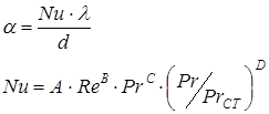 [4.26]
 [4.27]
 [4.28]
 [4.31]
 [4.32]
 [4.33]
 [4.34]
 [4.35]
 [4.36]
 - dispersion of an average;
 [4.37]
 - adequacy dispersion.
 [4.38]
 [4.39]
 [4.40]
 – mean square deviation of coefficient of regression.
 [4.41]
 [4.42]
 [4.43]
 [4.44]
 [4.45]
 [4.46]
 , ppm [4.47]
 , ppm [4.48]
 [4.49]