Заглавная страница Избранные статьи Случайная статья Познавательные статьи Новые добавления Обратная связь FAQ Написать работу КАТЕГОРИИ: ТОП 10 на сайте Приготовление дезинфицирующих растворов различной концентрацииТехника нижней прямой подачи мяча. Франко-прусская война (причины и последствия) Организация работы процедурного кабинета Смысловое и механическое запоминание, их место и роль в усвоении знаний Коммуникативные барьеры и пути их преодоления Обработка изделий медицинского назначения многократного применения Образцы текста публицистического стиля Четыре типа изменения баланса Задачи с ответами для Всероссийской олимпиады по праву 
Мы поможем в написании ваших работ! ЗНАЕТЕ ЛИ ВЫ?
Влияние общества на человека
Приготовление дезинфицирующих растворов различной концентрации Практические работы по географии для 6 класса Организация работы процедурного кабинета Изменения в неживой природе осенью Уборка процедурного кабинета Сольфеджио. Все правила по сольфеджио Балочные системы. Определение реакций опор и моментов защемления |
Consumer preferences and consumer choiceСодержание книги
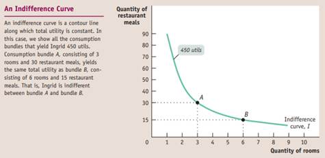
Поиск на нашем сайте An indifference curve is a line that shows all the consumption bundles that yield the same amount of total utility for an individual.
The entire utility function of an individual can be represented by an indifference curve map, a collection of indifference curves in which each curve corresponds to a different total utility level. Properties of Indifference Curves No two individuals have the same indifference curve map because no two individuals have the same preferences. But economists believe that, regardless of the person, every indifference curve map has two general properties: ■ Indifference curves never cross. Suppose that we tried to draw an indifference curve map like the one depicted in the left diagram in panel (a), in which two indifference curves cross at A. What is the total utility at A? Is it 100 utils or 200 utils? Indifference curves cannot cross because each consumption bundle must correspond to a unique total utility level—not, as shown at A, two different total utility levels. ■ The farther out an indifference curve lies—the farther it is from the origin—the higher the level of total utility it indicates. The reason, illustrated in the right diagram in panel (a), is that we assume that more is better—we consider only the consumption bundles for which the consumer is not satiated. Bundle B, on the outer indifference curve, contains more of both goods than bundle A on the inner indifference curve. So B, because it generates a higher total utility level (200 utils), lies on a higher indifference curve than A. ■ Indifference curves slope downward. Here, too, the reason is that more is better. The left diagram in panel (b) shows four consumption bundles on the same indifference curve: W, X, Y, and Z. By definition, these consumption bundles yield the same level of total utility. But as you move along the curve to the right, from W to Z, the quantity of rooms consumed increases. The only way a person can consume more rooms without gaining utility is by giving up some restaurant meals. So the indifference curve must slope downward.
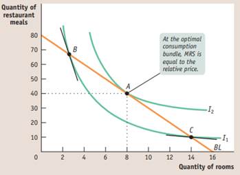
The marginal rate of substitution, or MRS, of good R in place of good M is equal to MUR/MUM, the ratio of the marginal utility of R to the marginal utility of M. The principle of diminishing marginal rate of substitution states that the more of good R a person consumes in proportion to good M, the less M he or she is willing to substitute for another unit of R. Two goods, R and M, are ordinary goods in a consumer’s utility function when (1) the consumer requires additional units of R to compensate for less M, and vice versa; and (2) the consumer experiences a diminishing marginal rate of substitution when substituting one good in place of another. The tangency condition between the indifference curve and the budget line holds when the indifference curve and the budget line just touch. This condition determines the optimal consumption bundle when the indifference curves have the typical convex shape.
The relative price of good R in terms of good M is equal to PR/PM, the rate at which R trades for M in the market. (QR × PR) + (QM × PM) = N Optimal consumption bundle: MUR/MUM=PR/PM Optimal consumption rule: MUR/PR=MUM/PM
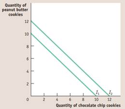
Two goods are perfect substitutes if the marginal rate of substitution of one good in place of the other good is constant, regardless of how much of each an individual consumes.
Two goods are perfect complements when a consumer wants to consume the goods in the same ratio regardless of their relative price.
The relationship between most goods for most people falls somewhere between these two extremes.
The change in a consumer’s optimal consumption bundle caused by a change in price can be decomposed into two effects: the substitution effect, due to the change in relative price, and the income effect, due to the change in purchasing power. The substitution effect refers to the substitution of the good that is now relatively cheaper in place of the good that is now relatively more expensive, holding the total utility level constant. It is represented by a movement along the original indifference curve. When a price change alters a consumer’s purchasing power, the resulting change in consumption is the income effect. It is represented by a movement to a different indifference curve, keeping the relative price unchanged. For normal goods, the income and substitution effects work in the same direction; so their demand curves always slope downward. Although these effects work in opposite directions for inferior goods, their demand curves usually slope downward as well because the substitution effect is typically stronger than the income effect. The exception is a Giffen good.
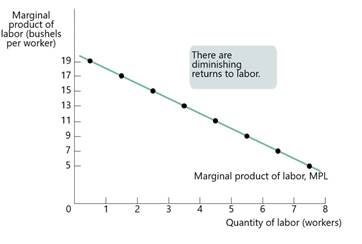
A production Function Is the relationship between the Q of inputs a firm uses and the Q of output it produces. A Fixed input is an input whose Q is fixed for a period of time and cannot be varied. A Variable input is an input whose Q the Firm can vary at any time. The long run is the time period in which all inputs can be varied. The short run is the time period in which at least one input is fixed. The total product curve shows how the Q of output depends on the Q of the variable input, for a given Q of the fixed input. The Marginal product of an input is the additional Q of output that is produced by using one more unit of that input.
There are diminishing returns to an input when an Increase in the Q of that input, holding the levels of all other inputs fixed, leads to a decline in the marginal product of that input.
The Total Cost of producing a given Q of output is the sum of the fixed cost and the variable cost of producing that quantity of output. TC=FC+VC The total cost curve becomes steeper as more output is produced due to diminishing returns.
As in the case of Marginal product, MC is equal to “rise” (the increase in TC) divided by “run” (the increase in the Q of output. Why is the MC curve upward sloping? -Because there are diminishing returns to inputs in this example. As output increases, the marginal product of the variable input declines. -This implies that more and more of the variable input must be used to produce each additional unit of output as the amount of output already produced rises. -And since each unit of the Variable input must be paid for, the cost per additional unit of output also rises. Average total cost, often referred to simply as average cost, is total cost divided by Q of output produced. ATC= TC/Q A U-shaped average total cost curve falls at low levels of output, then rises at higher levels. Average Fixed Cost is the fixed cost per unit of output. AFC= FC/Q Average variable cost is the variable cost per unit of output AVC= VC/Q Increasing output has two opposing effects on average total cost: - The spreading effect: the larger the output, the greater the Q of output over which FC is spread, leading to lower the AFC. - The diminishing returns effect: the larger the output, the greater the amount of variable input required to produce additional units leading to higher average variable cost.
The min cost output is the Q of output at which ATC is lowest – the bottom of U-shaped ATC curve. At the min cost output, ATC is equal to MC. At output less than the min-cost output, MC is less than ATC and ATC is falling. And an output greater than the min-cost output, MC is greater than ATC and ATC is rising. In the short run, fixed cost is completely outside the control of a firm. But all inputs are variable in the long run. The firm will choose its FC in the long run based on the level of output it expects to produce. The long run ATC curve shows the relationship between output and ATC when FC has been chosen to minimize ATC for each level of output. -there are increasing returns to scale when long-run ATC declines as output increases. -there are decreasing returns to scale when long run ATC increases as output increases. -there are constant returns to scale when long run ATC is constant as output increases. 1. The relationship between inputs and output is a producer's production function. In the short run, the quantity of a fixed input cannot be varied but the quantity of a variable input can. In the long run, the quantities of all inputs can be varied. For a given amount of the fixed input, the total product curve shows how the quantity of output changes as the quantity of the variable input changes. 2. There are diminishing returns to an input when its marginal product declines as more of the input is used, holding the quantity of all other inputs fixed. 3.Total cost is equal to the sum of fixed cost, which does not depend on output, and variable cost, which does depend on output. 4. Average total cost, total cost divided by quantity of output, is the cost of the average unit of output, and marginal cost is the cost of one more unit produced. U-shaped average total cost curves are typical, because average total cost consists of two parts: average fixed cost, which falls when output increases (the spreading effect), and average variable cost, which rises with output (the diminishing returns effect). 5. When average total cost is U-shaped, the bottom of the U is the level of output at which average total cost is minimized, the point of minimum- cost output. This is also the point at which the marginal cost curve crosses the average total cost curve from below. 6.In the long run, a producer can change its fixed input and its level of fixed cost. The long-run average total cost curve shows the relationship between output and average total cost when fixed cost has been chosen to minimize average total cost at each level of output. 7.As output increases, there are increasing returns to scale if long-run average total cost declines; decreasing returns to scale if it increases; and constant returns to scale if it remains constant. Scale effects depend on the technology of production.
|
||
|
|
Последнее изменение этой страницы: 2021-07-19; просмотров: 307; Нарушение авторского права страницы; Мы поможем в написании вашей работы! infopedia.su Все материалы представленные на сайте исключительно с целью ознакомления читателями и не преследуют коммерческих целей или нарушение авторских прав. Обратная связь - 216.73.216.119 (0.005 с.) |


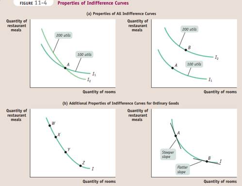 ■ Indifference curves have a convex shape. The right diagram in panel (b) shows that the slope of each indifference curve changes as you move down the curve to the right: the curve gets flatter. If you move up an indifference curve to the left, the curve gets steeper. So the indifference curve is steeper at A than it is at B. When this occurs, we say that an indifference curve has a convex shape—it is bowed-in toward the origin.
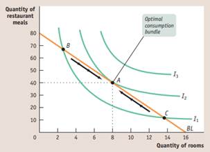


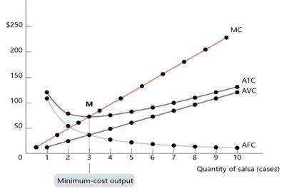 Putting the four cost curves together note that: MC is upward sloping due to diminishing returns; AVC also is upward sloping but is flatter than the MC curve; AFC is downward sloping because of the spreading effect; the MC curve intersects the ATC curve from below, crossing it at its lowest point.