Linear second-order equations with constant coefficients

Definition

A linear second-order ordinary differential equation with constant coefficients is a second-order ordinary differential equation that may be written in the form

x "(t) + ax '(t) + bx (t) = f (t)

for a function f of a single variable and numbers a and b. The equation is homogeneous if f (t) = 0 for all t.

Suppose that x and y are solutions of the equation

x "(t) + ax '(t) + bx (t) = f (t),

which we refer to subsequently as the “original equation”. Define z (t) = y (t) − x (t) for all t. Then z "(t) + az '(t) + bz (t) = [ y "(t) + ay '(t) + by (t)] − [ x "(t) + ax '(t) + bx (t)] = f (t) − f (t) = 0. That is, z is a solution of the homogeneous equation

x "(t) + ax '(t) + bx (t) = 0.

Conversely, let x be a solution of the original equation, let z be a solution of the homogeneous equation, and define y (t) = x (t) + z (t) for all t. Then y is a solution of original equation.

Thus we have the following result.

Proposition

Let x be a solution of the linear second-order ordinary differential equation with constant coefficients

x "(t) + ax '(t) + bx (t) = f (t).

Then y is a solution of this equation if and only if y (t) = x (t) + z (t) for all t, where z is a solution of the (homogeneous) equation

x "(t) + ax '(t) + bx (t) = 0.

The practical importance of this result is that the set of all solutions of the original equation may be found by finding one solution of this equation and adding to it the general solution of the homogeneous equation. That is, we may use the following procedure to solve the original equation.

Procedure for finding general solution of linear second-order ordinary differential equation with constant coefficients

The general solution of the differential equation

x "(t) + ax '(t) + bx (t) = f (t)

may be found as follows.

1. Find the general solution of the associated homogeneous equation x "(t) + ax '(t) + bx (t) = 0.

2. Find a single solution of the original equation x "(t) + ax '(t) + bx (t) = f (t).

3. Add together the solutions found in steps 1 and 2.

I now explain how to perform the first two steps and illustrate step 3.

1. Find the general solution of a homogeneous equation

You might guess, based on the solutions we found for first-order equations, that the homogeneous equation has a solution of the form x (t) = Ae^rt. Let's see if it does. If x (t) = Ae^rt then x '(t) = rAe^rt and x "(t) = r ² Ae^rt, so that

x "(t) + ax '(t) + bx (t)	=	r ^2 Ae^rt + arAe^rt + bAe^rt
	=	Ae^rt (r ^2 + ar + b).

Thus for x (t) to be a solution of the equation we need

r ² + ar + b = 0.

This equation is knows as the characteristic equation of the differential equation. If a ² > 4 b this equation has two distinct real roots, if a ² = 4 b it has a single real root, and if a ² < 4 b it has two complex roots.

Suppose that a ² > 4 b, so that the characteristic equation has two distinct real roots, say r and s. We have shown that both x (t) = Ae^rt and x (t) = Be^st, for any values of A and B, are solutions of the equation. Thus also x (t) = Ae^rt + Be^st is a solution. It can be shown, in fact, that every solution of the equation takes this form.

The cases in which the characteristic equation has a single real root (a ² = 4 b) or complex roots (a ² < 4 b) require slightly different analyses, with the following conclusions.

Proposition SOURCE

Consider the homogeneous linear second-order ordinary differential equation with constant coefficients

x "(t) + ax '(t) + bx (t) = 0.

The general solution of this equation depends on the character of the roots of the characteristic equation r ² + ar + b = 0 as follows.

Distinct real roots

If a ² > 4 b, in which case the characteristic equation has distinct real roots, say r and s, the general solution of the equation is

Ae^rt + Be^st.

Single real root

If a ² = 4 b, in which case the characteristic equation has a single root, say r, the general solution of the equation is

(A + Bt) e^rt,

where r = −(1/2) a is the root.

Complex roots

If a ² < 4 b, in which case the characteristic equation has complex roots, the general solution of the equation is

(A cos(β t) + B sin(β t)) e ^{α t},

where α = − a /2 and β = √(b − a ²/4). This solution may alternatively be expressed as

Ce ^{α t} cos(β t + ω),

where the relationships between the constants C, ω, A, and B are A = C cos ω and B = − C sin ω.

You may be asking yourself how it is possible that trigonometric functions (sin and cos) appear in the solutions. The answer lies in fact that

e^ix = cos x + i sin x for all x,

where i is the square root of −1. For details, see Boyce and DiPrima (1969), pp. 106–116.

Example

Consider the differential equation

x "(t) + x '(t) − 2 x (t) = 0.

The characteristic equation is

r ² + r − 2 = 0

so the roots are 1 and −2. That is, the roots are real and distinct. Thus the general solution of the differential equation is

x (t) = Ae^t + Be ^{−2 t} .

Example

Consider the differential equation

x "(t) + 6 x '(t) + 9 x (t) = 0.

The characteristic equation has a single real root, −3. Thus the general solution of the differential equation is

x (t) = (A + Bt) e ^{−3 t} .

Example

Consider the equation

x "(t) + 2 x '(t) + 17 x (t) = 0.

The characteristic roots are complex. We have a = 2 and b = 17, so α = −1 and β = 4. Thus the general solution of the differential equation is

[ A cos(4 t) + B sin(4 t)] e ^{− t} .

2. Find a solution of a nonhomogeneous equation

Consider the nonhomogeneous equation

x "(t) + ax '(t) + bx (t) = f (t).

If f (t) is a constant, say c, x (t) = c / b is a solution if b ≠ 0, x (t) = ct / a is a solution if b = 0 and a ≠ 0, and x (t) = ct ²/2 is a solution if a = b = 0. For other forms of f, a good technique to find a solution is to try a linear combination of f (t) and its first and second derivatives. If, for example, f (t) = 3 t − 6 t ², then f '(t) = 3 − 12 t and f "(t) = −12, so that you should try to find values of A, B, and C such that A + Bt + Ct ² is a solution. Or if f (t) = 2sin t + cos t, then you should try to find values of A and B such that f (t) = A sin t + B cos t is a solution. Or if f (t) = 2 e^Bt for some value of B, then you should try to find a value of A such that Ae^Bt is a solution.

Example

Consider the differential equation

x "(t) + x '(t) − 2 x (t) = t ².

A linear combination of the function on the right-hand side and its first and second derivatives is C + Dt + Et ². For this function to be a solution,

2 E + D + 2 Et − 2 C − 2 Dt − 2 Et ² = t ² for all t.

For this condition to be satisfied (note that the equation must be satisfied for all t), the constant and coefficient of t on the left must be zero and the coefficient of t ² on the left must be 1. That is,

2 E + D − 2 C	= 0
2 E − 2 D	= 0
−2 E	= 1.

The unique solution of these equations is E = −1/2, D = −1/2, and C = −3/4. Thus

x (t) = −3/4 − t /2 − t ²/2

is a solution of the differential equation.

3. Add together the solutions found in steps 1 and 2

This step is quite trivial!

Example

Consider the equation from the previous example, namely

x "(t) + x '(t) − 2 x (t) = t ².

We saw above that the general solution of the associated homogeneous equation is

x (t) = Ae^t + Be ^{−2 t} .

and that

x (t) = −3/4 − t /2 − t ²/2

is a solution of the original equation.

Thus the general solution of the original equation is

x (t) = Ae^t + Be ^{−2 t} − 3/4 − t /2 − t ²/2.

Second-order initial value problems

A first-order initial value problem consists of a first-order ordinary differential equation x '(t) = F (t, x (t)) and an “initial condition” that specifies the value of x for one value of t. For a second-order equation, requiring an initial condition of that form does not generally determine a unique solution. To determine a unique solution, we generally need to specify both the value of x for some value of t and the rate of change of x at that value of t. Accordingly, we make the following definition.

Definition

A second-order initial value problem consists of a second-order ordinary differential equation

x "(t) = F (t, x (t), x '(t))

and initial conditions

x (t ₀) = x ₀ and x '(t ₀) = k ₀

where t ₀, x ₀, and k ₀ are numbers.

Example

Consider the second-order initial value problem in which the differential equation is the one in theprevious example, namely

x "(t) + x '(t) − 2 x (t) = t ²,

and the initial conditions are

x (0) = 0 and x '(0) = 1.

From the previous example, the general solution of the equation is

x (t) = Ae^t + Be ^{−2 t} − 3/4 − t /2 − t ²/2.

We have

x (0)	=	A + B − 3/4
x '(0)	=	A − 2 B − 1/2

so that for the initial conditions to be satisfied we need

	=	A + B − 3/4
	=	A − 2 B − 1/2.

The unique solution of these equations is A = 1, B = −1/4. Thus the solution of the initial value problem is

x (t) = e^t − (1/4) e ^{−2 t} − 3/4 − t /2 − t ²/2.

Equilibrium and stability

The notions of equilibrium and stability for a second-order initial value problem are closely related to the corresponding notion for a first-order initial value problem.

Definition

If for some initial conditions a second-order initial value problem has a solution that is a constant, the value of the constant is an equilibrium or stationary state of the associated differential equation. If, for all initial conditions, the solution of a second-order initial value problem converges to an equilibrium of the associated differential equation as the variable t increases without bound, then the equilibrium is globally stable.

Consider the homogeneous linear second-order equation

x "(t) + ax '(t) + bx (t) = 0.

If b ≠ 0, this equation has a single equilibrium, namely 0. (That is, the only constant function that is a solution is equal to 0 for all t.) To study the stability of this equilibrium, consider separately the three possible forms of the general solution of the equation, as given in a previous result.

Characteristic equation has two real roots

If the characteristic equation has two real roots, r and s, the general solution of the equation is Ae^rt + Be^st. This function converges to 0 for all values of A and B, so that the equilibrium is globally stable, if and only if r < 0 and s < 0.

Characteristic equation has a single real root

If the characteristic equation has a single real root, r, the general solution of the equation is (A + Bt) e^rt. This function converges to 0 for all values of A and B, so that the equilibrium is globally stable, if and only if r < 0. (If r < 0 then for any value of k, t^ke^rt converges to 0 as t increases without bound.)

Characteristic equation has complex roots

If the characteristic equation has complex roots, the general solution of the equation is (A cos(β t) + B sin(β t)) e ^{α t}, where α = − a /2, β = √(b − a ²/4). This function converges to 0 for all values of A and B, so that the equilibrium is globally stable, if and only if α < 0, or equivalently a > 0. (Remember that cos θ and sin θ lie between +1 and −1 for all values of θ.)

Now, the roots of the characteristic equation

r ² + ar + b = 0

are, by the quadratic formula,

(− a ± √(a ² − 4 b))/2.

Thus if these roots are complex, then the real part of each of them is − a /2. Hence the condition for stability in the case of complex roots is that the real part of each root is negative. Because the real part of a real root is simply the root, the conditions in the other two cases are exactly the same. That is, regardless of the nature of the roots, the equilibrium is globally stable if and only if the real part of each root of the characteristic equation is negative.

If b = 0, then every number is an equilibrium. By a previous result the general solution of the equation is Ae ^{− at} + B if a ≠ 0 and A + Bt if a = 0. In both cases, for no equilibrium does the solution converge to the equilibrium for all values of A and B.

Thus an equilibrium of the second-order linear homogeneous equation

x "(t) + ax '(t) + bx (t) = 0

is globally stable if and only if the real parts of each root of the characteristic equation

r ² + ar + b = 0

is negative. If a ² > 4 b then the roots are real, equal to (− a ± √(a ² − 4 b))/2. They are both negative if − a + √(a ² − 4 b) < 0, which is true if and only if a > 0 and b > 0. If a ² = 4 b then b ≥ 0 (because the square of any number is nonnegative) and the single root is − a /2, which is negative if and only if a > 0, in which case b > 0. Finally, if a ² < 4 b then also b > 0 and the real part of each root is − a /2, which is negative if and only if a > 0.

Thus we have the following result.

Proposition

An equilibrium of the homogeneous linear second-order ordinary differential equation with constant coefficients x "(t) + ax '(t) + bx (t) = 0 is stable if and only if the real parts of both roots of thecharacteristic equation r ² + ar + b = 0 are negative, or, equivalently, if and only if a > 0 and b > 0.

Now consider the (nonhomogeneous) linear second-order equation

x "(t) + ax '(t) + bx (t) = c

where b ≠ 0 and c ≠ 0. The constant function x (t) = c / b is a solution of this equation, so that by ourprocedure, the general solution of the equation is the sum of c / b and the general solution of the homogeneous equation

x "(t) + ax '(t) + bx (t) = 0.

Thus the equilibrium (0) of this homogeneous equation is globally stable if and only if the equilibrium of the original equation is globally stable. That is, we have the following result.

Proposition

For any value of c, an equilibrium of the linear second-order ordinary differential equation with constant coefficients x "(t) + ax '(t) + bx (t) = c with b ≠ 0 is stable if and only if the real parts of both roots of thecharacteristic equation r ² + ar + b = 0 are negative, or, equivalently, if and only if a > 0 and b > 0.

Example

Consider the following macroeconomic model. Denote by Q aggregate supply, p the price level, and π the expected rate of inflation. Assume that aggregate demand is a linear function of p and π, equal to a − bp + c π where a > 0, b > 0, and c > 0. An equilibrium condition is

Q (t) = a − bp (t) + c π(t).

Denote by Q * the long-run sustainable level of output (a constant), and assume that prices adjust according to the equation

p '(t) = h (Q (t) − Q *) + π(t),

where h > 0. Finally, suppose that expectations are adaptive:

π'(t) = k (p '(t) − π(t))

for some k > 0. Is the equilibrium of this system stable?

One way to answer this question is to reduce the system to a single second-order differential equation by differentiating the equation for p '(t) to obtain p "(t) and then substituting in for π'(t) and π(t). We obtain

p "(t) − h (kc − b) p '(t) + khbp (t) = kh (a − Q *).

Given k > 0, h > 0, and b > 0, we have khb > 0, so from the previous proposition the equilibrium is stable if and only if kc < b.

In particular, if c = 0 (i.e. expectations are ignored) then the equilibrium is stable. If expectations are taken into account, however, and respond rapidly to changes in the rate of inflation (k is large), then the equilibrium may not be stable.

 

11 lecture

 

 

Random events and their properties. The full group of random events. Classical statistical and geometric probability. Addition theorems of probability of joint and incompatible events. Independent random events.

 

 

Geometric Probability

Random events that take place in continuous sample space may invoke geometric imagery for at least two reasons: due to the nature of the problem or due the the nature of the solution.

Some problems, like Buffon's needle, Birds On a Wire, Bertrand's Paradox, or the problem of the Stick Broken Into Three Pieces do, by their nature, arise in a geometric setting. The latter also admits multiple reformulations which require comparison of the areas of geometric figures. In general, we may think of geometric probabilities as non-negative quantities (not exceeding 1) being assigned to subregions of a given domain subject to certain rules. If function μ is an expression of this assignment defined on a domain D, then, for example, we require

0 ≤ μ(A) ≤ 1, A ⊂ D and
μ(D) = 1

The function μ is usually not defined for all A ⊂ D. Those subsets of D for which μ is defined are the random events that form a particular sample spaces. Very often μ is defined by means of the ratio of areas so that, if σ(A) is defined as the "area" of set A, then one may set μ(A) = σ(A) / σ(D).

Problem 1

Two friends who take metro to their jobs from the same station arrive to the station uniformly randomly between 7 and 7:20 in the morning. They are willing to wait for one another for 5 minutes, after which they take a train wether together or alone. What is the probability of their meeting at the station?

In a Cartesian system of coordinates (s, t), a square of side 20 (minutes) represents all the possibilities of the morning arrivals of the two friends at the metro station.

The gray area A is bounded by two straight lines, t = s + 5 and t = s - 5, so that inside A, |s - t| ≤ 5. It follows that the two friends will meet only provided their arrivals s and t fall into region A. The probability of this happening is given by the ratio of the area of A to the are of the square:

[400 - (15×15/2 + 15×15/2)] / 400 = 175/400 = 7/16.

Problem 2

([ Sveshnikov, problem 3.12].)

Three points A, B, C are placed at random on a circle of radius 1. What is the probability for ΔABC to be acute?.

Fix point C. The positions of points A and B are then defined by arcs α and β extending from C in two directions. A priori we know that 0 < α + β < 2π. The favorable for our problem values of α and β (as subtending acute angles satisfy) 0 < α < π and 0 < β < π. Their sum could not be less than π as this would make angle C obtuse, therefore,α + β > π. The situation is presented in the following diagram where the square has the side 2π.

Region D is the intersection of three half-planes: 0 < α, 0 < β, and α + β < 2π. This is the big triangle in the above diagram. The favorable events belong to the shaded triangle which is the intersection of the half-planes α < π, β < π,and α + β > π. The ratio of the areas of the two is obviously 1/4.

Now observe, that unless the random triangle is acute it can be thought of as obtuse since the probability of two of the three points A, B, C forming a diameter is 0. (For BC to be a diameter, one should have α + β = π which is a straight line, with zero as the only possible assignment of area.) Thus we can say that the probability of ΔABC being obtuse is 3/4. For an obtuse triangle, the circle can be divided into two halves with the triangle lying entirely in one of the halves. It follows that 3/4 is the answer to the following question:

 

 

12 lecture

 

 

Conditional probability. Theorem of multiplication of probabilities. The formula of total probability. Bayes' formula.

 

 

 

 

 

 

 

13 lecture

 

 

Elements of linear programming. Graphical method.

 

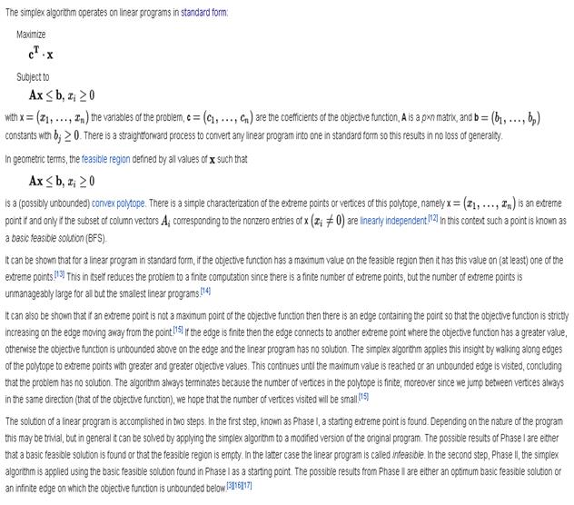
Graphical Method

The graphical method for solving linear programming problems in two unknowns is as follows.

1. Graph the feasible region.
2. Compute the coordinates of the corner points.
3. Substitute the coordinates of the corner points into the objective function to see which gives the optimal value. This point gives the solution to the linear programming problem.
4. If the feasible region is not bounded, this method can be misleading: optimal solutions always exist when the feasible region is bounded, but may or may not exist when the feasible region is unbounded.

If the feasible region is unbounded, we are minimizing the objective function, and its coefficients are non-negative, then a solution exists, so this method yields the solution.

To determine if a solution exists in the general unbounded case:

1. Bound the feasible region by adding a vertical line to the right of the rightmost corner point, and a horizontal line above the highest corner point.
2. Calculate the coordinates of the new corner points you obtain.
3. Find the corner point that gives the optimal value of the objective function.
4. If this optimal value occurs at a point of the original (unbounded) region, then the LP problem has a solution at that point. If not, then the LP problem has no optimal solution.

Example

Minimize C = 3 x + 4 y subject to the constraints

3 x - 4 y ≤ 12,
x + 2 y ≥ 4
x ≥ 1, y ≥ 0.

The feasible region for this set of constraints was shown above. Here it is again with the corner points shown.

Although the feasible region is unbonded, we are minimizing C = 3 x + 4y, whose coefficients are non-negative, and so the method shown above left applies.

The following table shows the value of C at each corner point:

Point	C = 3 x + 4y
(1, 1.5)	3(1)+4(1.5) = 9	minimum
(4, 0)	3(4)+4(0) = 12

Therefore, the solution is x = 1, y = 1.5, giving the minimum value C = 9.

 

 

14 lecture

 

Simplex method. The algorithm of the Simplex method.

 

 

 

 

 

15 lecture

 

The transportation problem. Finding the initial of the support solutions.

 

 

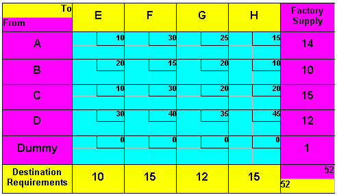
The Transportation Problem

There is a type of linear programming problem that may be solved using a simplified version of the simplex technique called transportation method. Because of its major application in solving problems involving several product sources and several destinations of products, this type of problem is frequently called the transportation problem. It gets its name from its application to problems involving transporting products from several sources to several destinations. Although the formation can be used to represent more general assignment and scheduling problems as well as transportation and distribution problems. The two common objectives of such problems are either (1) minimize the cost of shipping m units to n destinations or (2) maximize the profit of shipping m units to n destinations.

Let us assume there are m sources supplying n destinations. Source capacities, destinations requirements and costs of material shipping from each source to each destination are given constantly. The transportation problem can be described using following linear programming mathematical model and usually it appears in a transportation tableau.

There are three general steps in solving transportation problems.

We will now discuss each one in the context of a simple example. Suppose one company has four factories supplying four warehouses and its management wants to determine the minimum-cost shipping schedule for its weekly output of chests. Factory supply, warehouse demands, and shipping costs per one chest (unit) are shown in Table 7.1

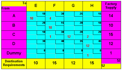
Table 7.1 ”Data for Transportation Problem”

At first, it is necessary to prepare an initial feasible solution, which may be done in several different ways; the only requirement is that the destination needs be met within the constraints of source supply.

The Transportation Matrix

The transportation matrix for this example appears in Table 7.2, where supply availability at each factory is shown in the far right column and the warehouse demands are shown in the bottom row. The unit shipping costs are shown in the small boxes within the cells (see transportation tableau – at the initiation of solving all cells are empty). It is important at this step to make sure that the total supply availabilities and total demand requirements are equal. Often there is an excess supply or demand. In such situations, for the transportation method to work, a dummy warehouse or factory must be added. Procedurally, this involves inserting an extra row (for an additional factory) or an extra column (for an ad warehouse). The amount of supply or demand required by the ” dummy ” equals the difference between the row and column totals.

In this case there is:

Total factory supply … 51

Total warehouse requirements … 52

This involves inserting an extra row - an additional factory. The amount of supply by the dummy equals the difference between the row and column totals. In this case there is 52 – 51 = 1. The cost figures in each cell of the dummy row would be set at zero so any units sent there would not incur a transportation cost. Theoretically, this adjustment is equivalent to the simplex procedure of inserting a slack variable in a constraint inequality to convert it to an equation, and, as in the simplex, the cost of the dummy would be zero in the objective function.

 

Table 7.2 "Transportation Matrix for Chests Problem With an Additional Factory (Dummy)"

 

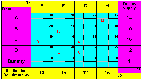
Initial Feasible Solution

Initial allocation entails assigning numbers to cells to satisfy supply and demand constraints. Next we will discuss several methods for doing this: the Northwest-Corner method, Least-Cost method, and Vogel's approximation method (VAM).

Table 7.3 shows a northwest-corner assignment. (Cell A-E was assigned first, A-F second, B-F third, and so forth.) Total cost: 10*10 + 30*4 + 15*10 + 30*1 + 20*12 + 20*2 + 45*12 + 0*1 = 1220($).

Inspection of Table 7.3 indicates some high-cost cells were assigned and some low-cost cells bypassed by using the northwest-comer method. Indeed, this is to be expected since this method ignores costs in favor of following an easily programmable allocation algorithm.

Table 7.4 shows a least-cost assignment. (Cell Dummy-E was assigned first, C-E second, B-H third, A-H fourth, and so on.) Total cost: 30*3 + 25*6 + 15*5 +10*10 + 10*9 + 20*6 + 40*12 + 0*1= 1105 ($).

Table 7.5 shows the VAM assignments. (Cell Dummy-G was assigned first, B-F second, C-E third, A-H fourth, and so on.) Note that this starting solution is very close to the optimal solution obtained after making all possible improvements (see next chapter) to the starting solution obtained using the northwest-comer method. (See Table 7.3.) Total cost: 15*14 + 15*10 + 10*10 + 20*4 + 20*1 + 40*5 + 35*7 + 0*1 = 1005 ($).

Table 7.3 ”Northwest – Corner Assignment”

Table 7.4"Least - Cost Assignment"

 

Table 7.5 "VAM Assignment"

Develop Optimal Solution

To develop an optimal solution in a transportation problem involves evaluating each unused cell to determine whether a shift into it is advantageous from a total-cost stand point. If it is, the shift is made, and the process is repeated. When all cells have been evaluated and appropriate shifts made, the problem is solved. One approach to making this evaluation is the Stepping stone method.

The term stepping stone appeared in early descriptions of the method, in which unused cells were referred to as "water" and used cells as "stones"— from the analogy of walking on a path of stones half-submerged in water. The stepping stone method was applied to the VAM initial solution, as shown in Table 7.5

Table 7.6 shows the optimal solutions reached by the Stepping stone method. Such solution is very close to the solution found using VAM method.

Table 7.6 "Optimal Matrix, With Minimum Transportation Cost of $1,000."

Alternate Optimal Solutions

When the evaluation of any empty cell yields the same cost as the existing allocation, an alternate optimal solution exists (see Stepping Stone Method – alternate solutions). Assume that all other cells are optimally assigned. In such cases, management has additional flexibility and can invoke nontransportation cost factors in deciding on a final shipping schedule.

Table 7.7 "Alternate Optimal Matrix for the Chest Transportation Problem, With Minimum Transportation Cost of $1,000.

Degeneracy

Degeneracy exists in a transportation problem when the number of filled cells is less than the number of rows plus the number of columns minus one (m + n - 1). Degeneracy may be observed either during the initial allocation when the first entry in a row or column satisfies both the row and column requirements or during the Stepping stone method application, when the added and subtracted values are equal. Degeneracy requires some adjustment in the matrix to evaluate the solution achieved. The form of this adjustment involves inserting some value in an empty cell so a closed path can be developed to evaluate other empty cells. This value may be thought of as an infinitely small amount, having no direct bearing on the cost of the solution.

Procedurally, the value (often denoted by the Greek letter epsilon, - ) is used in exactly the same manner as a real number except that it may initially be placed in any empty cell, even though row and column requirements have been met by real numbers. A degenerate transportation problem showing a Northwest Corner initial allocation is presented in Table 7.8, where we can see that if were not assigned to the matrix, it would be impossible to evaluate several cells.

Once a has been inserted into the solution, it remains there until it is removed by subtraction or until a final solution is reached.

While the choice of where to put an is arbitrary, it saves time if it is placed where it may be used to evaluate as many cells as possible without being shifted.

Table 7.8 "Degenerate Transportation Problem With Added. Number of filled cells = 4”

7.6 Transportation Problem with a Maximization as a Criterion

A fictive corporation A has a contract to supply motors for all tractors produced by a fictive corporation B. Corporation B manufactures the tractors at four locations around Central Europe: Prague, Warsaw, Budapest and Vienna. Plans call for the following numbers of tractors to be produced at each location:

Prague 9 000

Warsaw 12 000

Budapest 9 000

Corporation A has three plants that can produce the motors. The plants and production capacities are

Hamburg 8 000

Munich 7 000

Leipzig 10 000

Dresden 5 000

Due to varying production and transportation costs, the profit earns on each motor depends on where they were produced and where they were shipped. The following transportation table (Table 7.9) gives the accounting department estimates of the euro profit per unit (motor).

Table 7.9 "The Euro Profit Per One Shipped Motor"

Table 7.10 shows a highest - profit assignment (Least Cost method modification). In contrast to the Least – Cost method it allocates as much as possible to the highest-cost cell. (Cell Hamburg - Budapest was assigned first, Munich - Warsaw second, Leipzig - Warsaw third, Leipzig – Budapest fourth, Dresden – Prague fifth and Leipzig – Prague sixth.) Total profit: 3 335 000 euro.

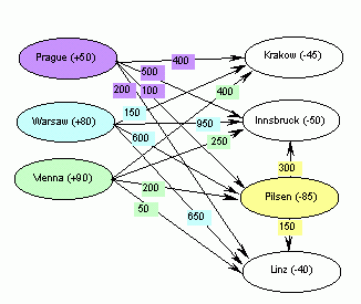
Table 7.10 "Highest - Profit Assignment"

Applying the Stepping Stone method (modified for maximization purposes) to the initial solution we can see that no other transportation schedule can increase the profit and so the Highest – Profit initial allocation is also an optimal solution of this transportation problem.

The Transshipment Problem

The transshipment problem is similar to the transportation problem except that in the transshipment problem it is possible to both ship into and out of the same node (point). For the transportation problem, you can ship only from supply points to demand points. For the transshipment problem, you can ship from one supply point to another or from one demand point to another. Actually, designating nodes as supply points or demand points becomes confusing when you can ship both into and out of a node. You can make the designations clearer if you classify nodes by their net stock position-excess (+), shortage (-), or 0.

One reason to consider transshipping is that units can sometimes be shipped into one city at a very low cost and then transshipped to other cities. In some situations, this can be less expensive than direct shipment.
Let's consider the balanced transportation problem as an example.

Picture 7.1 shows the net stock positions for the three warehouses and four customers. Say that it is possible to transship through Pilsen to both Innsbruck and Linz. The transportation cost from Pilsen to Innsbruck is 300 euro per unit, so it costs less to ship from Warsaw to Innsbruck by going through Pilsen. The direct cost is 950 euro, and the transshipping cost is 600 + 300 = 900 euro. Because the transportation cost is 300 euro from Pilsen to Innsbruck, the cost of transshipping from Prague through Pilsen to Innsbruck is 400 euro per unit. It is cheaper to transship from Prague through Pilsen than to ship directly from Prague to Innsbruck.

Picture 7.1 "Transshipment Example in the Form of a Network Model"

There are two possible conversions to a transportation model. In the first conversion, make each excess node a supply point and each shortage node a demand point. Then, find the cheapest method of shipping from surplus nodes to shortage nodes considering all transshipment possibilities. Let's perform the first conversion for the Picture 7.1 example. Because a transportation table Prague, Warsaw, and Vienna have excesses, they are the supply points. Because Krakow, Pilsen, Innsbruck, and Linz have shortages, they are the demand points. The cheapest cost from Warsaw to Innsbruck is 900 euro, transshipping through Pilsen. The cheapest cost from Prague to Innsbruck is 400 euro, transshipping through Pilsen too. The cheapest cost from all other supply points to demand points is obtained through direct shipment. Table 7.11 shows the balanced transportation table for this transshipment problem. For a simple transportation network, finding all of the cheapest routes from excess nodes to shortage nodes is easy. You can list all of the possible routes and select the cheapest. However, for a network with many nodes and arcs, listing all of the possible routes is difficult.

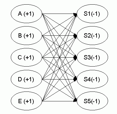
Table 7.11 "The Transshipment Problem After Conversion to a Transportation Model"

The second conversion of a transshipment problem to a transportation model doesn't require finding all of the cheapest routes from excess nodes table to shortage nodes. The second conversion requires more supply and demand nodes than the first conversion, because the points where you can ship into and out of, occur in the converted transportation problem twice – first as a supply point and second as a demand point.

The Assignment Problem

Another transportation problem is the assignment problem. You can use this problem to assign tasks to people or jobs to machines. You can also use it to award contracts to bidders. Let's describe the assignment problem as assigning n tasks to n people. Each person must do one and only one task, and each task must be done by only one person. You represent each person and each task by a node. Number the people 1 to n, and number the tasks 1 to n. The assignment problem can be described simply using a verbal model or using a linear programming mathematical model.

For example, say that five groups of computer users must be trained for five new types of software. Because the users have different computer skill levels, the total cost of trainings depends on the assignments.

Table 7.12 ”Cost of Trainings According to the Groups of Users”

Picture 7.2 "Network Model for Assignment Problem"

Table 7.12 shows the cost of training for each assignment of a user group (A through E) to a software type (S1 through S5). Picture 7.2 is a network model of this problem.

A balanced assignment problem has the same number of people and tasks. For a balanced assignment problem, the relationships are all equal. Each person must do a task. For an unbalanced assignment problem with more people than tasks, some people don't have to do a task and the first class of constraints is of the type. In general, the simplex method does not guarantee that the optimal values of the decision variables are integers. Fortunately, for the assignment model, all of the corner point solutions have integer values for all of the variables. Therefore, when the simplex method determines the optimal corner point, all of the variable values are integers and the constraints require that the integers be either 1 or 0 (Boolean).