Заглавная страница Избранные статьи Случайная статья Познавательные статьи Новые добавления Обратная связь КАТЕГОРИИ: ТОП 10 на сайте Приготовление дезинфицирующих растворов различной концентрацииТехника нижней прямой подачи мяча. Франко-прусская война (причины и последствия) Организация работы процедурного кабинета Смысловое и механическое запоминание, их место и роль в усвоении знаний Коммуникативные барьеры и пути их преодоления Обработка изделий медицинского назначения многократного применения Образцы текста публицистического стиля Четыре типа изменения баланса Задачи с ответами для Всероссийской олимпиады по праву 
Мы поможем в написании ваших работ! ЗНАЕТЕ ЛИ ВЫ?
Влияние общества на человека
Приготовление дезинфицирующих растворов различной концентрации Практические работы по географии для 6 класса Организация работы процедурного кабинета Изменения в неживой природе осенью Уборка процедурного кабинета Сольфеджио. Все правила по сольфеджио Балочные системы. Определение реакций опор и моментов защемления |
Scheme of laboratory research facility
4) Table of measuring instruments:
5) Equations for calculations: 1. Total power: PT [mW]= I [mA] × e, where I – current; e – EMF of the source. 2. Useful power: PU [mW]=I2·R ·10 3, where R – resistance of load resistor. 3. Efficiency: η = (РU / РT)·100 %. 1) Table of measurements: R=R3; e =UV = … V, when I =Imin (or R3=9 999 W).
7) Calculation of quantities:
9) Conclusions: 9a) With increasing of load resistance the total power … 9b) With increasing of load resistance the efficiency … 9c) Useful power has a …, when …, therefore optimal mode with greatestdelivery to external resistance corresponds to load matching condition …. 10) Data: “___” _____20___. Work done by: ______ Work checked by: ( Surname, readable) LABORATORY WORK № 3-1 Topic: STIDYING MAGNETIC FIELD VIA TANGENT-COMPASS
2. Goal of the work: 2.1. Study of method of a vector diagrams for representation of magnetic field. 2.2. Finding the horizontal component of a magnetic intensity vector in the laboratory via tangent-compass. Main concepts 3.1. Magnetic field of currents. Intensity and induction of magnetic field Any moving electric charge creates a magnetic field. Electric current (as an ordered motion of charges) creates a magnetic field too. Magnetic field around a permanent magnet is being created by orientation in one direction of atomic micro-currents of material of magnet. In the magnetic field other moving charge (or current) experiences a force. Thus wires with parallel currents are being attracted and with anti-parallel are being repulsed, because the magnetic field of moving charges of first wire acts on moving charges of the second wire. As the objects of interaction in magnetism usually consider or moving electric charges or elements of current. Element of the current Idl – is aproduct of a current I and infinitesimal segment of wire dl. Element of current is a vector, whose direction coincides with direction of the current. Element of current in Magnetism is similar to test charge in Electrostatics – it is a probe with the help of which we can explore magnetic field. As it has been established by Ampere, any element of the current, placed in a magnetic field B, will experience a force:
Note that the direction of Ampere’s force doesn’t coincide with that of vector of magnetic induction Quantity
Equation (84) gives us a definition of magnetic induction:
Vector of magnetic induction numerically equals to force, with which magnetic field acts on a unit element of current (I × dl = 1 A×m), placed perpendicularly to vector of magnetic induction (when
SI unit for 1 T = 1 N / 1 A×m. Graphically magnetic field can be depicted with the help of magnetic field lines (lines of magnetic force). Magnetic field lineis a type of line for which the tangent line to the path at each point is parallel to the vector
In order to determine direction of vector B the corkscrew rule (Fig. 24) is used: if translational motion of screw coincides with current I, then rotational motion point out a direction of magnetic field lines B.
Each element of a current generates a magnetic field around it. Induction of that field defines by Biot-Savart-Laplace law:
here, r – is the distance between the element of a current Idl and the point A at which the field induction Quantity If we divide equation (86) on mm0 we’ll obtain quantity, which is independent from properties of medium – magnetic intensity:
Equation (87) is a Biot-Savart-Laplace law for magnetic intensity. It defines the value of magnetic field intensity dH for the field, generated by element of the current Idl. Therefore a definition of magnetic intensity:
The SI unit for magnetic intensity is ampere per meter. Directions of If wire has a complex shape (see fig. 25) it can be represented as a huge number of elements of current Idl. Resultant magnetic intensity (or induction) at any point is a vector sum of elementary intensities
This superposition principle allows determine intensity (or induction) of field, created by wires with different form. Magnetic intensity characterizes only magnetic field of macroscopic currents, because it don’t depend on magnetic properties of medium. Now, let’s consider some special cases.
3.1.1. Finite segment of current create a circular magnetic field (Fig.26). Magnetic intensity at a distance of r from axis of a current defined with the formula:
here r – a1 and a2 - angles, which are created radius-vectors, traced from the ends of a conductor to the target point A at which field is being calculated. Vectors of magnetic intensity Magnetic field lines are concentric circles around a straight current which are lying in perpendicular plane to a current. Direction of field lines can be determined by the corkscrew rule (Fig. 26): if translational motion of screw coincides with current I, then rotational motion point out a direction of magnetic field lines H.
3.1.2. Infinite straight current create a magnetic fieldsame as a segment (Fig. 27).
If length of a segment (Fig.26) increases then angles α1 and α2 will decrease until they become zero as in the case of infinite wire. As cos 0° = 1, then НA = I / 2p r. (90)
Direction of
3.1.3. Circular current (single coil)(Fig.28). Magnetic intensity at the center of a circular current can be defined with the formula Н C = I / 2 R, (91)
here, R – is the radius of a circle. Vector Intensity magnitude on the axis of the circle can be defined with the formula H A = IR 2 / 2 (R+h) 3 / 2, (92) where h – distance from the point in which the field is being calculated to the center of coil. 3.1.4. Solenoid. (Fig.29) is a wire, wound around a cylindrical core. Length of a solenoid is in many times greater than its diameter. Inside the solenoid magnetic field there is uniform with intensity H = IN / l = I×n, (93)
where, N - number of loops of wire in a solenoid, l –solenoids length, n – number of loops per unit length(winding density). Uniformity of a field is broken at ends of solenoid. Outside there is a weak field with respect to an inside field. Direction of
3.1.5. Torus (Fig. 30) is a wire wound around a toroidal core. Torus has no boundary effect. Magnetic field is completely concentrated inside the torus, Н = IN / l = I×п, (93) here, l – is the length of midline of a torus. Earth’s magnetic field
The Earth is a natural magnet. In different points on the Earth there is a magnetic needle, able to swing around horizontal and vertical axis, sets under the different angles with Earth’s surface. It means that field lines and vector of intensity have different angles with its surface. The magnetic poles are the two positions on Earth's surface where the magnetic field is entirely vertical. There magnetic needle sets vertically. Magnetic field S pole is near the Earth's geographic North Pole and the other magnetic field N pole is near the Earth's geographic South Pole. The exact positions of geographical and magnetic poles don’t coincide. The locations of the magnetic poles are not static; they wander as much as 15 km every year. As it is seen from Fig. 31, the field lines come out of the Earth on the south hemisphere, and come in on the north one. Vertical plane, which is drawn through magnetic needle, is called magnetic meridian plane. Line of intersection of this plane with Earth’s surface is known as magnetic meridian. In other words, magnetic meridian is the line, connecting the magnetic south and north poles. The angle between the magnetic and the geographic meridian is the magnetic declination j. The angle between vector of intensity and horizontal plane is the magnetic inclination i. Vector of intensity can be decomposed on two components – horizontal
Magnitude of
|
||||||||||||||||||||||||||||||||||||||||||||||||||||||||||||||||||||||||||||||||||||||||||||||||||||||||||||||||||||||
|
|
Последнее изменение этой страницы: 2016-04-26; просмотров: 64; Нарушение авторского права страницы; Мы поможем в написании вашей работы! infopedia.su Все материалы представленные на сайте исключительно с целью ознакомления читателями и не преследуют коммерческих целей или нарушение авторских прав. Обратная связь - 3.133.137.17 (0.026 с.) |


 , or, in scalars,
  . (84)
 Fig. 23–Left hand rule
 . Its direction defines by a “ left hand rule ”: if you place left hand so that four fingers point the direction of current (see Fig. 23), and vector of magnetic induction
  =>
=>  ; [ B ]= T. (85)
 ).
). Fig. 24–Corkscrew (right-hand screw) rule
 , or, in scalars,
  , (86)
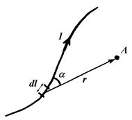 Fig. 25 – Illustration to the
Biot-Savart-Laplace law
Fig. 25 – Illustration to the
Biot-Savart-Laplace law
 is being computed (Fig. 25); m0=4p∙10–7 H / m – magnetic constant (permeability of vacuum); m – relative permeability of medium, it shows in what many times induction in a given medium is different from that of vacuum.
 . (87)
 . [ H ]=
  . (88)
 coincide only in isotropic homogeneous medium or in nonmagnetic material.
 (or inductions
  ) of fields created by each element of current Idl individually:
 ;
;  .
. , (89)
 Fig. 26 – Field lines of segment of a current and corkscrew rule
 Fig. 27 – Field lines of an infinite current
 Fig. 28 – Field lines of a circular current
 is perpendicular to the plane of a coil in each point underlying in a plane of that coil. It can be derived from superposition principle applied to set of magnetic fields produced by each segment of wire dl separately.
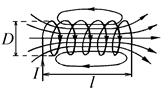 Fig. 29 – Field lines of solenoid
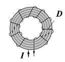 Fig. 30 – Torus
 Fig. 31 – Earth’s magnetic field lines
 and vertical –
  (Fig. 32). The magnetic needle, able to swing randomly in horizontal plane, will point its north pole in the direction of
  . Magnetic declination, magnetic inclination, and magnitude of horizontal component of magnetic field intensity completely characterize Earth’s magnetic field.
 Fig. 32 – Two components of Earth’s magnetic field intensity
 of Earth’s magnetic field determine with the help of tangent-compass in different points of laboratory desktop.