Заглавная страница Избранные статьи Случайная статья Познавательные статьи Новые добавления Обратная связь КАТЕГОРИИ: ТОП 10 на сайте Приготовление дезинфицирующих растворов различной концентрацииТехника нижней прямой подачи мяча. Франко-прусская война (причины и последствия) Организация работы процедурного кабинета Смысловое и механическое запоминание, их место и роль в усвоении знаний Коммуникативные барьеры и пути их преодоления Обработка изделий медицинского назначения многократного применения Образцы текста публицистического стиля Четыре типа изменения баланса Задачи с ответами для Всероссийской олимпиады по праву 
Мы поможем в написании ваших работ! ЗНАЕТЕ ЛИ ВЫ?
Влияние общества на человека
Приготовление дезинфицирующих растворов различной концентрации Практические работы по географии для 6 класса Организация работы процедурного кабинета Изменения в неживой природе осенью Уборка процедурного кабинета Сольфеджио. Все правила по сольфеджио Балочные системы. Определение реакций опор и моментов защемления |
Ministry of education and science of ukraineСтр 1 из 10Следующая ⇒
MINISTRY OF EDUCATION AND SCIENCE OF UKRAINE
ODESSA NATIONAL ACADEMY OF TELECOMMUNICATIONS after A. S. POPOV ====================================================================== Department of physics of optical communications
PHYSICS Module 1. Electrical current and magnetic field of a current ELECTROMAGNETISM PART 3: LABORATORY WORKS for bachelor training of educational area 6.050903 –“Telecommunications”
ODESSA 2015 UDK 538 (075.8) Publication plan 2015e.
Writers: assoc. prof. Gorbachov V.E, instructor Kardashev K.D., Tumbrukati E.G.
The following methodical guide is about section “Electromagnetism” of physics course for telecommunications technician. Four laboratory works allow students to learn basics of electrical engineering and measuring technique applied to determine main characteristics of electrical systems and magnetic field. It contains sufficient theoretical information combined with detailed descriptions of applied electromagnetic equipment construction such as Whetstone bridge, tangent-compass, and measuring techniques such as bridge circuit, comparison method. Recommended for students of TE-group, educational area 0924 –“Telecommunications”.
CONFIRMED at the Methodical council of ONAC Protocol № 9/14 from 19.15.2014e.
MODULE STRUCTURE Module № 1. „ Electrical current and magnetic field of a current” – 72 hours total Lectures – 16 hrs, pract. trainings – 0 hrs, labs – 16 hrs, self-studies – 33 hrs.
LIST OF LABORATORY WORKS
INTRODUCTION All laboratory works are provided in a frontal way, i.e. all group makes the same laboratory work at the same time. Appropriate homework must forego to work in a lab. The homework contains self-studying of theory and methodology of work accomplishment, preparation of protocol which includes experimental facility’s schematic drawing, equipment table's drawing, measurement table's drawing, a list of working formulae with description of all quantities which are in, list of control questions' answering. The allowance to performing of laboratory work will be had only those of students who have fulfilled homework and have positive result on express mini-quiz in a lab.
The report of each laboratory work should contain following steps: 1) Title and number of laboratory work. 2) Goal of the work. 3) Laboratory research facility's scheme. 4) Equipment table. 5) Equations for calculation with decryption of all quantities in. 6) Standard table of measurements for each measured quantity. It has to be checked and verified by an instructor. 7) Experimental data processing (write one for many similar) 8) Standard form of result (confidence interval and relative error or a graphic result) 9) Conclusion 10) Date, name of a student.
Besides this guide is recommended to use literature from bibliography given at the end of this guide. Далее Лаб 2.1 и 3.4 Абзац отступ 1,25 Формулы 14 дпи Надписи к рисункам 12 дпи
Нумерация разделов и рисунков Тире – длинные LABORATORY WORK № 2-1 Topic: STUDYING OF ELECTROSTATIC FIELD 2. Goal of the work: 2.1. Study the main characteristics of electrostatic field: intensity, potential and relation between them. 2.2. Investigation of electrostatic field with the help of equipotential surfaces. Main concepts Test questions 1. What is an electric intensity? What are the units of measurement of the electric intensity? What is the direction of the electric intensity? 2. How to calculate electric intensity of:, an infinite uniformly charged plate, an infinite uniformly charged thread, a point charge? 3. What is the potential of the field in a given point? What are the units of potential? 4. How the work of the electric field forces does defines through the potential difference? 5. What is the field line? Draw the field lines of: positive and negative point charges, plane, and thread. 6. What is equipotential surface? Draw equipotential surfaces of: a plane, a thread, a point charge. 7. What is the relation between intensity and potential? 8. How can in the lab we experimentally find the location of equipotential surfaces? Draw a scheme. 9. How can we calculate the intensity of the field in point between the equipotential lines? Content of the report Equipment table
5) Quantities calculation formulae:
Table of measurements
7) Quantities calculation:
8) Final result: (Exemplary diagram of distribution of potential and electric field lines)
Experimentally obtained (!!!) diagram (or its copy) with measurements has to be pasted in a protocol. 9) Conclusion: On the experimentally obtained space distribution of a potential we have counted the vectors of … in various points of electric field. 10) Data: “___” _____20___. Work done by: ______ Work checked by: ( Surname, readable) LABORATORY WORK № 2-2 BRIDGE 2. Goal of the work: 2.1. Study the method of measurements by means of a bridge circuit. 2.2. Study the method of data processing. 2.3. Finding a resistance of conductors.
Main concepts Kirchhoff’s rules For a solution of branched circuits it is used two rules, which are algorithm for set up of equations that relate currant, voltages, and electromotive forces on elements of branched circuit. Before usage of Kirchhoff’s rules for solution of branched circuit, for example, of bridge circuit (see Fig. 11), we should assign three topological elements of the circuit: Junction – is a point of connection of three or greater conductors. On Fig. 11 junctions are marked by letters A, B, C and D. Branch – is a way from one junction to a neighbour junction with its own elements. One's own current flows in each branch from initial junction to end junction through all elements of this branch. Therefore the branch's number usually same as the current's number.
For example, on Fig. 11 we see: current I 1 flows through branch AD, current I 2 flows through branch DС, current I 3 flows through branch BС, current I 4 flows through branch AB, current I 5 flows through branch CA, current I 6 flows through branch BD. If in the branch we have a source of EMF, then direction of current should coincide with direction of extraneous forces work (from “–“ to “+” inside the source). If in the branch a source is absent, direction of current should be set any way.
Closed loop – is a way from a junction to the same junction with its own elements. For each considered closed loop it is necessary to choose at once directions of path-tracing (or clockwise, or against) and to fix on the circuit schema. For example, on Fig. 11: the trace direction of loops ADCA and ABCA is chosen anticlockwise. 1st Kirchhoff’s rule – is a junction’s rule:
where 2nd Kirchhoff’s rule – is a closed loop’s rule:
Data processing For representation of the result of direct measurements of quantity x it is necessary: 1) Obtain the sequence of data x 1, x 2, x 3, ..., xn (reduce to a Table of measurements). 2) Calculate the average value of measurand:
3) Find an abmodality each measurement (in a Table of measurements):
4) Square each abmodality and summarize (in a Table of measurements):
5) Find a statistical absolute error of measurements from Sdudent’s equation:
where a – confidence probability; n – number of measurements; t a; n – Sdudent’s coefficient. 6) Find a device absolute error of measurements
b - accuracy class of electrical measuring instrument, х max – grid limit. 7) Find a total absolute error of measurements D x = 7) Calculate relative error of measurements:
8) Final result is represented by a confidence interval and relative error:
For representation of the result of indirect measurements of quantity y it is necessary: 1) Calculate the average value of measurand < y > by formula from average values of known quantities < a >, < b >, < c >, for example:
2) Calculate relative error of measurand d y from relative errors of known quantities d a , d b , d c by formula that should be gained accordingly to this example:
where D a, D b, D c – absolute errors of known quantities; < a >, < b >, < c > – its average values. 3) Find an absolute error of measurand D y = < y >×d y. (51) 4) Final result should be represented by a confidence interval and relative error:
Test questions 1. What are the SI units for resistance? 2. What parametres of a conductor define its resistance? 3. How it is possible to define a total resistance in serial and parallel connections of resistors? 4. Draw the scheme of Wheatstone bridge. 5. What is the point of Wheatstone bridge method of measurements of resistance? 6. Derive the relation between resistances of bridge's arms at balance with Ohm’s law. 7. Derive the relation between resistances of bridge's arms at balance with Kirchhoff‘s laws. 8. How it is possible to calculate statistical absolute error and device absolute error of measurements. Content of the report
Homework toLaboratory work №2-2 (Answers on test questions from p.26) … BRIDGE 2) Goal: 1. Study the method of measurements by means of a bridge circuit. 2. Study the method of data processing. 3. Finding a resistance of resistor.
4) Table of measuring instruments:
5) Equations for calculation: 5.1) At the ballance condition I mA=0 of Wheatstone bridge the unknown resistance:
5.2) Statistical absolute error of measurements:
where a =0,95 – confidence probability; n=5 – number of measurements; t 0,95; 5= 2,77 – Sdudent’s coefficient. 5.3) Device absolute error of measurements:
where 5.4) Total absolute error of measurements:
5.5) Relative error of measurements
6) Table of measurements: R1 =10 k W = 10000 W;
7) Quantities calculation: … 7.1) Calculation of unknown resistance:
7.2) Calculation of statistical absolute error of measurements of resistance:
7.3) Calculation of device absolute error of measurements of resistance:
7.4) Calculation of total absolute error and relative error of measurements:
8) Final results: Rx = (<Rx> ±DRx) aW = (... ± ...)0,95 W; 9) Conclusions: At measuring of unknown resistance by means of a most accurate method of Wheatstone bridge the basic contribution to an absolute error has introduced … (ststistical or device) error. 10) Data: “___” _____20___. Work done by: ______ Work checked by: ( Surname, readable) LABORATORY WORK № 2-3 Main concepts In point 2.2 ofMain concepts of lab № 2-1 have been given definitions of a potential (11) and potential differences (14) as basic performances of an electric field. Definitions ofmagnitude of the EMF of a source, a voltage drop and voltage will be below given. Data processing (Same as in Laboratory work № 2-2). Compensation method 1. Mount the scheme Fig. 19. As a modelling source of the EMF we choose a source e1, which is on the left side of a laboratory board. In series with it we connect one-decade resistors box R 2, which simulates the sources internal resistance. Auxiliary source e2 is on the right side of a laboratory board. 2. Turn on both observable and auxiliary sources. Set the value R 2=0, thus 3. Set the potentiometer slider in the middle. Lock the switches К 1 and then К 2. 4. 5. Only at the moment of compensation we can write down the voltmeter scale reading eXi into a measurements table. To disconnect switches К 1 and К 2. 6. To set sequentially values of resistance of one-decade resistors box R 2 equal 10 kW, 30 kW, 50 kW, 70 kW, thus 7. Calculate average value of EMF <eX> (41), abmodality each measurement DeXi (42), sum of squares of abmodalities 8. For known the sum of squares of abmodalities calculate statistical absolute error DeXST (44) for confidence probability a=0,95, number of measurements n =5 and Sdudent’s coefficient 9. Calculate absolute device error DeXDEV according (45):
where b - accuracy class and U max – grid limit of voltmeter. 10. Calculate total absolute error De (46) and relative error de (47) of measurements. 11. Write a final result as a confidence interval and relative error (48). 12. Conclude about valuess of statistical and device absolute errors. 5.2. Direct method 1. Mount the scheme Fig. 18. As a modelling source of the EMF we choose a source e1, which is on the left side of a laboratory board. Resistors box R 2 simulate the sources internal resistance. 2. Turn on observable source. Set the value R 2=0, thus 3. Write down the voltmeter scale reading Ui into a measurements table. 4. To set sequentially values of resistance of resistors box R 2 equal 10 kW, 30 kW, 50 kW, 70 kW, 90 kW, thus 5. Calculate a relative error 6. Represent the final result by a draph of dependence error of direct method of measurements β i DIR from relative value of internal resistance of a source rXi / RV . 7. Conclude about range of values of internal resistances of source at which measuring it is possible to consider correct (when the value of error of direct method of measurements b i DIR is less). Test questions 1. What is potential, voltage (potential difference), EMF of the source, voltage drop?
2. How does Ohm's law look for uniform part of circuit, for non-uniform part of circuit, for the closed circuit? 3. When do potentials difference on the terminals of the source is equal to its EMF? 4. What is compensation method of measurement EMF of sources? Draw the scheme. 5. How the voltage between the points of the circuit can be calculated, if all EMFs of all sources and resistances of all parts of the circuit are known? 6. What is compensated in a compensation method of measuring of the EMF? Draw the scheme.
Content of the report
Homework toLaboratory work №2-3 (Answers on test questions from p.14) … LABORATORY WORK № 2-4 Main concepts Data processing The results of this laboratory work must be presented in a graphical aspect - is a plot of dependence of total and useful powers also efficiency of the source versus a load resistance. The graphical form of results usually guesses quality estimation and consequently does not demand statistical manipulation.
Test questions 1. What are total power, useful power, and efficiency of a source? 2. Derive a formula of total power dependence on external resistance. Analyze the obtained formula. Build the graph. What values of external resistance do they equal zero with? Are there maximal values? 3. Derive a formula of useful power dependence on external resistance. Analyze an obtained formula. Build a graph. 4. Derive what value of external resistance useful power is maximal with? 5. Derive a formula of efficiency dependence on external resistance. Analyze an obtained formula. Build a graph. 6. Write formulas of total power, useful power and efficiency dependencies on a current. What value of a current useful power is maximal with? 7. What are unuseful mode, power-saving mode and optimal mode with greatestdelivery to external resistance? Content of the report
LABORATORY WORK № 3-1 Main concepts 3.1. Magnetic field of currents. Intensity and induction of magnetic field Any moving electric charge creates a magnetic field. Electric current (as an ordered motion of charges) creates a magnetic field too. Magnetic field around a permanent magnet is being created by orientation in one direction of atomic micro-currents of material of magnet. In the magnetic field other moving charge (or current) experiences a force. Thus wires with parallel currents are being attracted and with anti-parallel are being repulsed, because the magnetic field of moving charges of first wire acts on moving charges of the second wire. As the objects of interaction in magnetism usually consider or moving electric charges or elements of current. Element of the current Idl – is aproduct of a current I and infinitesimal segment of wire dl. Element of current is a vector, whose direction coincides with direction of the current. Element of current in Magnetism is similar to test charge in Electrostatics – it is a probe with the help of which we can explore magnetic field. As it has been established by Ampere, any element of the current, placed in a magnetic field B, will experience a force:
Note that the direction of Ampere’s force doesn’t coincide with that of vector of magnetic induction Quantity
Equation (84) gives us a definition of magnetic induction:
Vector of magnetic induction numerically equals to force, with which magnetic field acts on a unit element of current (I × dl = 1 A×m), placed perpendicularly to vector of magnetic induction (when
SI unit for 1 T = 1 N / 1 A×m. Graphically magnetic field can be depicted with the help of magnetic field lines (lines of magnetic force). Magnetic field lineis a type of line for which the tangent line to the path at each point is parallel to the vector
In order to determine direction of vector B the corkscrew rule (Fig. 24) is used: if translational motion of screw coincides with current I, then rotational motion point out a direction of magnetic field lines B.
Each element of a current generates a magnetic field around it. Induction of that field defines by Biot-Savart-Laplace law:
here, r – is the distance between the element of a current Idl and the point A at which the field induction
Quantity If we divide equation (86) on mm0 we’ll obtain quantity, which is independent from properties of medium – magnetic intensity:
Equation (87) is a Biot-Savart-Laplace law for magnetic intensity. It defines the value of magnetic field intensity dH for the field, generated by element of the current Idl. Therefore a definition of magnetic intensity:
The SI unit for magnetic intensity is ampere per meter. Directions of If wire has a complex shape (see fig. 25) it can be represented as a huge number of elements of current Idl. Resultant magnetic intensity (or induction) at any point is a vector sum of elementary intensities
This superposition principle allows determine intensity (or induction) of field, created by wires with different form. Magnetic intensity characterizes only magnetic field of macroscopic currents, because it don’t depend on magnetic properties of medium. Now, let’s consider some special cases.
3.1.1. Finite segment of current create a circular magnetic field (Fig.26). Magnetic intensity at a distance of r from axis of a current defined with the formula:
here r – a1 and a2 - angles, which are created radius-vectors, traced from the ends of a conductor to the target point A at which field is being calculated. Vectors of magnetic intensity Magnetic field lines are concentric circles around a straight current which are lying in perpendicular plane to a current. Direction of field lines can be determined by the corkscrew rule (Fig. 26): if translational motion of screw coincides with current I, then rotational motion point out a direction of magnetic field lines H.
3.1.2. Infinite straight current create a magnetic fieldsame as a segment (Fig. 27). If length of a segment (Fig.26) increases then angles α1 and α2 will decrease until they become zero as in the case of infinite wire. As cos 0° = 1, then НA = I / 2p r. (90)
Direction of
3.1.3. Circular current (single coil)(Fig.28). Magnetic intensity at the center of a circular current can be defined with the formula Н C = I / 2 R, (91)
here, R – is the radius of a circle. Vector Intensity magnitude on the axis of the circle can be defined with the formula H A = IR 2 / 2 (R+h) 3 / 2, (92) where h – distance from the point in which the field is being calculated to the center of coil. 3.1.4. Solenoid. (Fig.29) is a wire, wound around a cylindrical core. Length of a solenoid is in many times greater than its diameter. Inside the solenoid magnetic field there is uniform with intensity H = IN / l = I×n, (93)
where, N - number of loops of wire in a solenoid, l –solenoids length, n – number of loops per unit length(winding density). Uniformity of a field is broken at ends of solenoid. Outside there is a weak field with respect to an inside field. Direction of
3.1.5. Torus (Fig. 30) is a wire wound around a toroidal core. Torus has no boundary effect. Magnetic field is completely concentrated inside the torus, Н = IN / l = I×п, (93) here, l – is the length of midline of a torus. Earth’s magnetic field
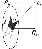
The Earth is a natural magnet. In different points on the Earth there is a magnetic needle, able to swing around horizontal and vertical axis, sets under the different angles with Earth’s surface. It means that field lines and vector of intensity have different angles with its surface. The magnetic poles are the two positions on Earth's surface where the magnetic field is entirely vertical. There magnetic needle sets vertically. Magnetic field S pole is near the Earth's geographic North Pole and the other magnetic field N pole is near the Earth's geographic South Pole. The exact positions of geographical and magnetic poles don’t coincide. The locations of the magnetic poles are not static; they wander as much as 15 km every year. As it is seen from Fig. 31, the field lines come out of the Earth on the south hemisphere, and come in on the north one. Vertical plane, which is drawn through magnetic needle, is called magnetic meridian plane. Line of intersection of this plane with Earth’s surface is known as magnetic meridian. In other words, magnetic meridian is the line, connecting the magnetic south and north poles. The angle between the magnetic and the geographic meridian is the magnetic declination j. The angle between vector of intensity and horizontal plane is the magnetic inclination i. Vector of intensity can be decomposed on two components – horizontal
Magnitude of
Data processing (Same as in Laboratory work № 2-2). Test questions 1. What is magnetic field induction? 2. What is magnetic field intensity? 3. What are the magnetic field lines? 4. Draw field lines for a circular current. How to determine direction of intensity vector in the center of a circular current? 5. Write the formula for calculation of intensity in the center and on the axis of circular current. 6. What are the main features of magnetic field lines with respect to electrostatic field lines? 7. What is superposition principle? How the resultant magnetic intensity can be determined if the elementary intensities of each of elements of current are given. 8. How to determine the direction and magnitude of horizontal component of Earth’s magnetic field intensity by tangent-compass? Draw a scheme. Derive a calculation formula.
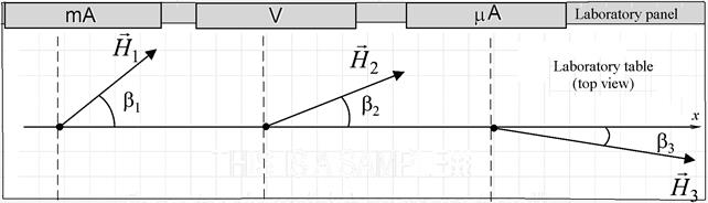
Content of the report VIA THE TANGENT-COMPASS 2) Goal: 1 Study of method of a vector diagrams for representation of force fields. 2 Finding the horizontal component of a magnetic field intensity vector in the laboratory via tangent-compass. 3) Scheme of laboratory research facility:
4) Table of measuring instruments:
5) Equations for calculations: Horizontal component of Earth’s magnetic field
where I – a current through the coil of tangent-compass; N – number of winds of a coil; D – diameter of a coil; a – angle of deviation of a needle when the current turn on from its zero-current position. Table of measurements N = 100; D = … mm.
7) Final results as a diagram:
8) Conclusions:
10) Data: “___” _____20___. Work done by: ______ Work checked by: ( Surname, readable)
LABORATORY WORK №3-4 Main concepts Diamagnetism The orbital motion of electrons creates tiny atomic current loops, which produce magnetic fields. When an external magnetic field is applied to a material, these current loops will tend to align in such a way as to oppose the applied field. Materials in which this effect is the only magnetic response are called diamagnetic. All materials are inherently diamagnetic, but if the atoms have some net magnetic moment as in paramagnetic materials, or if there is long-range ordering of atomic magnetic moments as in ferromagnetic materials, these stronger effects are always dominant. Diamagnetism is the residual magnetic behavior when materials are neither paramagnetic nor ferromagnetic. Any conductor will show a strong diamagnetic effect in the presence of changing magnetic fields because circulating currents will be generated in the conductor to oppose the magnetic field changes. A superconductor will be a perfect diamagnet since there is no resistance to the forming of the current loops. Paramagnetism Some materials exhibit a magnetization which is proportional to the applied magnetic field in which the material is placed. These materials are said to be paramagnetic. Paramagnetism is a form of magnetism which occurs only in the presence of an externally applied magnetic field. Paramagnetic materials are attracted to magnetic fields, hence have a relative magnetic permeability µ greater than one. The force of attraction generated by the applied field is linear in the field strength and rather weak. It typically requires a sensitive analytical balance to detect the effect. Paramagnets do not retain any magnetization in the absence of an externally applied magnetic field, because thermal motion causes the spins to become randomly oriented without it. Thus the total magnetization will drop to zero when the applied field is removed. Even in the presence of the field there is only a small induced magnetization because only a small fraction of the spins will be oriented by the field. This fraction is proportional to the field strength and this explains the linear dependency. Ferromagnetism Iron, nickel, cobalt and some of the rare earths (gadolinium, dysprosium) exhibit a unique magnetic behavior which is called ferromagnetism because iron (ferrum in Latin) is the most common and most dramatic example. Samarium and neodymium in alloys with cobalt have been used to fabricate very strong rare-earth magnets. Ferromagnetic materials exhibit a long-range ordering phenomenon at the atomic level which causes the unpaired electron spins to line up parallel with each other in a region called a domain. Within the domain, the magnetic field is intense, but in a bulk sample the material will usually be unmagnetized because the many domains will themselves be randomly oriented with respect to one another. Ferromagnetism manifests itself in the fact that a small externally imposed magnetic field, say from a solenoid, can cause the magnetic domains to line up with each other and the material is said to be magnetized. The driving magnetic field will then be increased by a large factor which is usually expressed as a relative permeability for the material. There are many practical applications of ferromagnetic materials, such as the electromagnet. Ferromagnets will tend to stay magnetized to some extent after being subjected to an external magnetic field. This tendency to "remember their magnetic history" is called hysteresis. The fraction of the saturation magnetization which is retained when the driving field is removed is called the remanence of the material, and is an important factor in permanent magnets. Ferromagntic materials will respond mechanically to an impressed magnetic field, changing length slightly in the direction of the applied field. This property, called magnetostriction, leads to the familiar hum of transformers as they respond mechanically to 60 Hz AC voltages. The long range order which creates magnetic domains in ferromagnetic materials arises from a quantum mechanical interaction at the atomic level. This interaction is remarkable in that it locks the magnetic moments of neighboring atoms into a rigid parallel order over a large number of atoms in spite of the thermal agitation which tends to randomize any atomic-level order. Sizes of domains range from a 0.1 mm to a few mm. When an external magnetic field is applied, the domains already aligned in the direction of this field grow at the expense of their neighbors. For a given ferromagnetic material the long range order abruptly disappears at a certain temperature which is called the Curie temperature for the material. In ferromagnetic materials the permeability µ depends on applied field and may be very large, up to 105. Hysteresis When a ferromagnetic material is magnetized in one direction, it will not relax back to zero magnetization when the imposed magnetizing field is removed. It must be driven back to zero by a field in the opposite direction. If an alternating magnetic field is applied to the material, its magnetization will trace out a loop called a hysteresis loop. The lack of retraceability of the magnetization curve is the property called hysteresis and it is related to the existence of magnetic domains in the material. Once the magnetic domains are reoriented, it takes some energy to turn them back again. This property of ferrromagnetic materials is useful as a magnetic "memory". Some compositions of ferromagnetic materials will retain an imposed magnetization indefinitely and are useful as "permanent magnets". The magnetic memory aspects of iron and chromium oxides make them useful in audio tape recording and for the magnetic storage of data on computer disks.
Hysteresis loop Data processing (Same as in Laboratory work № 2-2).
Test questions 1. What are the diamagnetics? 2. What are the paramagnetics? 3. What are the ferromagnetics? What their magnetization mechanism is? What is hysteresis phenomenon? Make a drawing of hysteresis loop and give explanations. 4. How the magnetic permeability of ferromagnet depends on magnetic field intensity magnitude? 5. Draw the scheme of lab 3-4. Derive magnetic field intensity magnitude formula which is used in this work. Derive magnetic induction magnitude formula which is used in this work Content of the report Table of measurements
7) Calculation of quantities and their errors 8) Graph (example! Do not redraw!!!):
9) Final results: 10) Conclusions: 10) Data: “___” _____20___. Work done by: ______ Work checked by: ( Surname, readable)
Bibliography
1. Трофимова Т. И. Курс физики. – М.: Высшая школа, 1990. 2. Зисман Г. А. и Тодес О. М. Курс общей физики – М. т. 2. § 14-17, 1974. 3. Детлаф А. А. Яворский Б. М. и др. Курс физики – М.; Высшая школа, т. 2, §9.1,.9.2, 9.4, 1977. 4. Калашников С. Г. Электричество. – М. Наука, §57, 58,59, 1977. 5. Викулин И. М. Электромагнетизм. Метод. указания для самостоятельной работы студентов по курсу физики. – Одесса: изд. УГАС, 2000.
1. Викулин И.М.Физика оптической связи: метод. указания для самост. работы студентов по курсу физики/ И.М.Викулин, В.Э.Горбачёв –Одесса: Од. міська друкарня, 2000. 2. Кучерук І.М.Загальний курс фізики: Т. III. Оптика. Квантова фізика/ І.М.Кучерук, І.Т.Горбачук – К.: Техніка, 1999. 3. Матвеев А.Н.Оптика/ А.Н.Матвеев –М.: Высшая школа, 1985. 4. Трофимова Т.Н.Курс физики/ Т.Н.Трофимова – М.: Высшая школа, 1985. 5. Зисман Г.А.Курс обшей физики. Т. III./ Г.А.Зисман, О.М. Тодес – М.: Наука, 1972. 6. Ландсберг Г.С. Оптика/ Г.С. Ландсберг – М.: Изд-во техн.-теорет. лит., 1957.
|
|||||||||||||||||||||||||||||||||||||||||||||||||||||||||||||||||||||||||||||||||||||||||||||||||||||||||||||||||||||||||||||||||||||||||||||||||||||||||||||||||||||||||||||||||||||||||||||||||||||||||||||||||||||||||||||||||||||||||||||||||||||||||||||||||||||||||||||||||||||||||||||||||||||||||
|
|
Последнее изменение этой страницы: 2016-04-26; просмотров: 49; Нарушение авторского права страницы; Мы поможем в написании вашей работы! infopedia.su Все материалы представленные на сайте исключительно с целью ознакомления читателями и не преследуют коммерческих целей или нарушение авторских прав. Обратная связь - 18.221.141.44 (0.393 с.) |


 ,
,
 ,
,
 – distance between the neighboring equipotential lines between which the value of an electric intensity has to be defined.
 ,
V
,
V


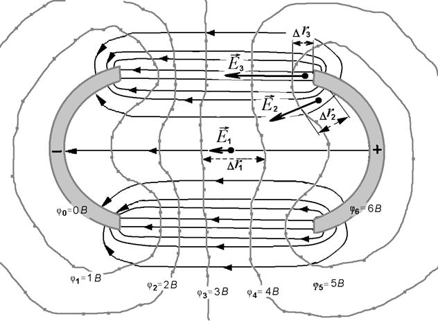
 Fig. 11 – Bridge’s branched circuit
 , (23)
 – algebraic sum of a current into the junction (which is positive when the currents flow in the junction, and negative when the currents flow out of the junction);
 , (24)
 – algebraic sum of voltage drops on external resistors around any closed loop, and
  – algebraic sum of the voltage drops on internal resistance of sources (which are positive, when the direction of a current coincides with chosen direction of path-tracing);
 – algebraic sum of the source electromotive force of the closed loop (which are positive, when the direction of extraneous forces work (from “–“ to “+” inside the source coincides with chosen direction of path-tracing).
 . (41)
 ;
;  ;...;
;...;  . (42)

 . (43)
 . (44)
 , (45)
 (46)
(46) . (47)
 = (… ± …)0.95;
  = … %. (48)
 . (49)
 , (50)
 = (… ± …)0.95;
  = … %. (52)
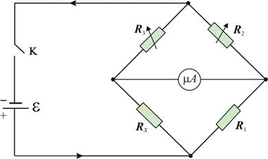
 .
. ,
, ,
, – average value of measurand; d – relative error of measurements; b i – accuracy class of electrical measuring instrument.
 .
. .
. =
=

 ;
;  ;
;  ;
; ;
;  .
. .
. .
. ;
; 
 = … %.
 .
. Moving the potentiometer slider, obtain absence of current through the microampermeter I =0.
 . It is equivalent to a changing of sources. Make measurements according to points 3, 4 and 5.
 (43).
(43). .
. ,
, (67) of each direct measurement (for each another sourse).
 , or, in scalars,
  . (84)
 Fig. 23–Left hand rule
 . Its direction defines by a “ left hand rule ”: if you place left hand so that four fingers point the direction of current (see Fig. 23), and vector of magnetic induction
  =>
=>  ; [ B ]= T. (85)
 ).
). Fig. 24–Corkscrew (right-hand screw) rule
 , or, in scalars,
  , (86)
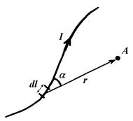 Fig. 25 – Illustration to the
Biot-Savart-Laplace law
Fig. 25 – Illustration to the
Biot-Savart-Laplace law
 is being computed (Fig. 25); m0=4p∙10–7 H / m – magnetic constant (permeability of vacuum); m – relative permeability of medium, it shows in what many times induction in a given medium is different from that of vacuum.
 . (87)
 . [ H ]=
  . (88)
 coincide only in isotropic homogeneous medium or in nonmagnetic material.
 (or inductions
  ) of fields created by each element of current Idl individually:
 ;
;  .
. , (89)
 Fig. 26 – Field lines of segment of a current and corkscrew rule
 Fig. 27 – Field lines of an infinite current
 Fig. 28 – Field lines of a circular current
 is perpendicular to the plane of a coil in each point underlying in a plane of that coil. It can be derived from superposition principle applied to set of magnetic fields produced by each segment of wire dl separately.
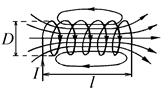 Fig. 29 – Field lines of solenoid
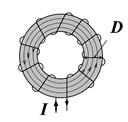 Fig. 30 – Torus
 Fig. 31 – Earth’s magnetic field lines
 and vertical –
  (Fig. 32). The magnetic needle, able to swing randomly in horizontal plane, will point its north pole in the direction of
  . Magnetic declination, magnetic inclination, and magnitude of horizontal component of magnetic field intensity completely characterize Earth’s magnetic field.
 Fig. 32 – Two components of Earth’s magnetic field intensity
 of Earth’s magnetic field determine with the help of tangent-compass in different points of laboratory desktop.
 ,
,